На русском языке
Acceleration
field
Acceleration field is a two-component vector field,
describing in a covariant way the four-acceleration
of individual particles and the four-force
that occurs in systems with multiple closely interacting particles. The
acceleration field is a component of the general
field, which is represented in the Lagrangian and Hamiltonian of an
arbitrary physical system by the term with the energy of particles’ motion and
the term with the field energy. [1] [2] The acceleration field is included in
most equations of vector field.
Moreover, the acceleration
field enters into the equation of motion through the acceleration tensor and into the equation
for the metric through the acceleration
stress-energy tensor.
The acceleration field was presented by Sergey Fedosin
within the framework of the metric theory
of relativity and
covariant theory of gravitation, and the
equations of this field were obtained as a consequence of the principle of
least action. [3] [4]
Contents
- 1 Mathematical description
- 1.1 Action, Lagrangian and energy
- 1.2 Equations
- 1.3 Stress-energy tensor
- 2 Specific solutions for acceleration field
functions
- 2.1 Ideally solid particle
- 2.2 Rotation of a particle
- 2.3 System of particles
- 3 Other approaches
- 4 The use in general theory of relativity
- 5 See also
- 6 References
- 7 External links
Mathematical description
The 4-potential of the
acceleration field is expressed in terms of the scalar ![]() and vector
and vector ![]() potentials:
potentials:
![]()
The antisymmetric acceleration tensor is calculated with the
help of the 4-curl of the 4-potential:
![]()
The acceleration tensor
components are the components of the field strength ![]() and the components of the solenoidal vector
and the components of the solenoidal vector ![]() :
:
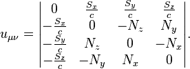
We obtain the following:
![]()
In the general case the scalar
and vector potentials are found by solving the wave equations for the
acceleration field potentials.
Action, Lagrangian and energy
In the covariant theory of gravitation the
4-potential ![]() of the acceleration field is part of the
4-potential of the general field
of the acceleration field is part of the
4-potential of the general field ![]() , which is the sum
of the 4-potentials of particular fields, such as the electromagnetic and
gravitational fields, acceleration field, pressure
field, dissipation field, strong
interaction field, weak interaction field and other vector fields, acting on
the matter and its particles. All of these fields are somehow represented in
the matter, so that the 4-potential
, which is the sum
of the 4-potentials of particular fields, such as the electromagnetic and
gravitational fields, acceleration field, pressure
field, dissipation field, strong
interaction field, weak interaction field and other vector fields, acting on
the matter and its particles. All of these fields are somehow represented in
the matter, so that the 4-potential ![]() cannot consist of only one 4-potential
cannot consist of only one 4-potential ![]() . The energy density of interaction of the general
field and the matter is given by the product of the 4-potential of the general
field and the mass 4-current:
. The energy density of interaction of the general
field and the matter is given by the product of the 4-potential of the general
field and the mass 4-current: ![]() . We obtain the
general field tensor from the 4-potential of the general field, using the
4-curl:
. We obtain the
general field tensor from the 4-potential of the general field, using the
4-curl:
![]()
The tensor invariant in the form ![]() is up to a
constant factor proportional to the energy density of the general field. As a
result, the action function, which contains the scalar curvature
is up to a
constant factor proportional to the energy density of the general field. As a
result, the action function, which contains the scalar curvature ![]() and the cosmological constant
and the cosmological constant ![]() , is given by the
expression: [1]
, is given by the
expression: [1]
![]()
where ![]() is the Lagrange function or Lagrangian;
is the Lagrange function or Lagrangian; ![]() is the time differential of the coordinate
reference system;
is the time differential of the coordinate
reference system; ![]() and
and ![]() are the constants to be determined;
are the constants to be determined; ![]() is the speed of light as a measure of the
propagation speed of the electromagnetic and gravitational interactions;
is the speed of light as a measure of the
propagation speed of the electromagnetic and gravitational interactions; ![]() is the invariant 4-volume expressed in terms
of the differential of the time coordinate
is the invariant 4-volume expressed in terms
of the differential of the time coordinate ![]() , the product
, the product ![]() of differentials of the space coordinates
and the square root
of differentials of the space coordinates
and the square root ![]() of the determinant
of the determinant
![]() of the metric
tensor, taken with a negative sign.
of the metric
tensor, taken with a negative sign.
The variation of the action
function gives the general field equations, the four-dimensional equation of
motion and the equation for the metric. Since the acceleration field is the
general field component, then from the general field equations the corresponding
equations of the acceleration field are derived.
Given the gauge condition of the
cosmological constant in the form
![]()
is met, the system energy does
not depend on the term with the scalar curvature and is uniquely determined: [4]
![]()
where ![]() and
and ![]() denote the time components of the
4-vectors
denote the time components of the
4-vectors ![]() and
and
![]() .
.
In an arbitrary reference frame K, the 4-momentum of a
system is determined by the formula: [5] [6]
![]()
where ![]() and
and ![]() denote the energy and momentum of the
physical system in K;
denote the energy and momentum of the
physical system in K; ![]() is the inertial mass;
is the inertial mass; ![]() is the 4-velocity of the center of momentum
of the physical system in K. If we place the origin of
coordinates of the reference frame K' at the center of momentum and calculate
in K' the energy of the system
is the 4-velocity of the center of momentum
of the physical system in K. If we place the origin of
coordinates of the reference frame K' at the center of momentum and calculate
in K' the energy of the system ![]() and the time component
and the time component ![]() of the 4-velocity of the center of momentum,
then we can find the inertial mass
of the 4-velocity of the center of momentum,
then we can find the inertial mass ![]() of the system. Note that in the reference
frame K' the three-dimensional momentum
of the system. Note that in the reference
frame K' the three-dimensional momentum ![]() of a physical system is by definition equal to zero.
of a physical system is by definition equal to zero.
Equations
The four-dimensional equations of the acceleration field
are similar in their form to Maxwell equations and are as follows:
![]()
![]()
where ![]() is the
mass 4-current,
is the
mass 4-current, ![]() is the mass density in the co-moving
reference frame,
is the mass density in the co-moving
reference frame, ![]() is the 4-velocity of the matter unit,
is the 4-velocity of the matter unit, ![]() is a constant, which is determined in each
problem, and it is supposed that there is an equilibrium between all fields in
the observed physical system.
is a constant, which is determined in each
problem, and it is supposed that there is an equilibrium between all fields in
the observed physical system.
The gauge condition of the
4-potential of the acceleration field:
![]()
If the second equation with the
field source is written with the covariant index in the following form:
![]()
then after substituting here the
expression for the acceleration tensor ![]() through the
4-potential
through the
4-potential ![]() of the
acceleration field we
obtain the wave equation for calculating the potentials of the acceleration
field: [7]
of the
acceleration field we
obtain the wave equation for calculating the potentials of the acceleration
field: [7]
![]()
where ![]() is the Ricci
tensor, found using the formula in the book. [8] If
the Ricci tensor is calculated using the formula in the book, [9] the
sign of the Ricci tensor in the wave equation should be reversed.
is the Ricci
tensor, found using the formula in the book. [8] If
the Ricci tensor is calculated using the formula in the book, [9] the
sign of the Ricci tensor in the wave equation should be reversed.
The continuity equation in curved
space-time is:
![]()
In Minkowski space
of the special theory of relativity, the Ricci tensor is set to zero, the form of the
acceleration field equations is simplified and they can be expressed in terms
of the field strength ![]() and the solenoidal vector
and the solenoidal vector ![]() :
:
![]()
![]()
where 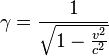 is the Lorentz factor,
 ![]() is the mass current density,
is the mass current density, ![]() is the velocity of the matter unit.
is the velocity of the matter unit.
The wave equation is also simplified and can be written separately for
the scalar and vector potentials:
![]()
![]()
The equation of motion of the
matter unit in the general field is given by the formula:
![]() .
.
Since ![]() , and the general field tensor is expressed in
terms of the tensors of particular fields, then the equation of motion can be
represented with the help of these tensors: [7] [10]
, and the general field tensor is expressed in
terms of the tensors of particular fields, then the equation of motion can be
represented with the help of these tensors: [7] [10]
![]()
Here ![]() is the electromagnetic tensor,
is the electromagnetic tensor, ![]() is the charge 4-current,
is the charge 4-current, ![]() is the gravitational
tensor,
is the gravitational
tensor, ![]() is the pressure
field tensor,
is the pressure
field tensor, ![]() is the dissipation
field tensor,
is the dissipation
field tensor, ![]() is the strong interaction field tensor,
is the strong interaction field tensor, ![]() is the weak interaction field tensor.
is the weak interaction field tensor. ![]() is invariant mass density,
is invariant mass density, ![]() and
and ![]() are the 4-velocity and 4-acceleration of the
matter unit.
are the 4-velocity and 4-acceleration of the
matter unit.
Stress-energy tensor
The acceleration
stress-energy tensor is calculated with the help of the acceleration
tensor:
![]() .
.
We find as part of the tensor ![]() the 3-vector of energy flux density of acceleration
field
the 3-vector of energy flux density of acceleration
field ![]() , which is similar
in its meaning to the Poynting vector and the Heaviside vector. The vector
, which is similar
in its meaning to the Poynting vector and the Heaviside vector. The vector ![]() can be represented through the vector product
of the field strength
can be represented through the vector product
of the field strength ![]() and the solenoidal vector
and the solenoidal vector ![]() :
:
![]()
here the index is ![]()
The covariant derivative of the
stress-energy tensor of the acceleration field with mixed indices specifies the 4-force density:
![]()
where ![]() denotes the proper time differential in the
curved spacetime.
denotes the proper time differential in the
curved spacetime.
The stress-energy tensor of the
acceleration field is part of the stress-energy tensor of the general field ![]() :
:
![]()
where ![]() is the electromagnetic stress–energy
tensor,
is the electromagnetic stress–energy
tensor, ![]() is the gravitational
stress-energy tensor,
is the gravitational
stress-energy tensor, ![]() is the pressure
stress-energy tensor,
is the pressure
stress-energy tensor, ![]() is the dissipation
stress-energy tensor,
is the dissipation
stress-energy tensor, ![]() is the strong interaction stress-energy
tensor,
is the strong interaction stress-energy
tensor, ![]() is the weak interaction stress-energy tensor.
is the weak interaction stress-energy tensor.
Through the tensor ![]() the stress-energy tensor of the acceleration
field enters into the equation for the metric:
the stress-energy tensor of the acceleration
field enters into the equation for the metric:
![]()
where ![]() is the Ricci tensor,
is the Ricci tensor, ![]() is the gravitational
constant,
is the gravitational
constant, ![]() is a certain constant, and the gauge
condition of the cosmological constant is used.
is a certain constant, and the gauge
condition of the cosmological constant is used.
Specific solutions for acceleration field functions
The four-potential of any vector field, the global vector potential of
which is equal to zero in the proper reference frame K', that is, in the
center-of-momentum frame, in case of rectilinear motion in the laboratory
reference frame K, can be presented as follows: [3] [7]
![]()
where ![]() is for the electromagnetic field and
is for the electromagnetic field and ![]() for the remaining fields;
for the remaining fields; ![]() and
and ![]() are the invariant mass density and the charge
density in the comoving reference frame, respectively;
are the invariant mass density and the charge
density in the comoving reference frame, respectively; ![]() is the invariant energy density of the interaction,
calculated as product of the four-potential of the field and the corresponding
four-current;
is the invariant energy density of the interaction,
calculated as product of the four-potential of the field and the corresponding
four-current; ![]() is the covariant four-velocity that
determines the motion of the center of momentum of the physical system in K.
is the covariant four-velocity that
determines the motion of the center of momentum of the physical system in K.
In the special relativity (SR), in the center-of-momentum frame K' the energy density
is ![]() ,
where
,
where ![]() is the Lorentz factor, and for the
acceleration field, while the physical system is moving in K, the
four-potential of the acceleration field will equal
is the Lorentz factor, and for the
acceleration field, while the physical system is moving in K, the
four-potential of the acceleration field will equal ![]() .
.
In case when the physical system is stationary in K, we will have ![]() , and consequently, the scalar potential will
be
, and consequently, the scalar potential will
be ![]() .
If in the physical system, on the average, there are directed fluxes of matter
or rotation of matter, the vector potential
.
If in the physical system, on the average, there are directed fluxes of matter
or rotation of matter, the vector potential
![]() of the acceleration field is no longer equal
to zero.
of the acceleration field is no longer equal
to zero.
If the
four-potential ![]() of acceleration field in K' is known, then in the laboratory
reference frame K the four-potential is determined using the matrix
of acceleration field in K' is known, then in the laboratory
reference frame K the four-potential is determined using the matrix ![]() connecting the coordinates and
time of both frames: [11]
connecting the coordinates and
time of both frames: [11]
![]()
In the
special case of the system’s motion at the constant velocity ![]() represents the Lorentz
transformation matrix.
represents the Lorentz
transformation matrix.
Ideally solid particle
In the approximation, when a particle
is regarded as an ideally solid object, the matter inside the particle is
motionless. It means that the Lorentz factor
![]() of this matter in the center-of-momentum frame K' is equal to unity, so that the
four-potential of the acceleration field becomes equal to the four-velocity of
motion of the center of momentum:
of this matter in the center-of-momentum frame K' is equal to unity, so that the
four-potential of the acceleration field becomes equal to the four-velocity of
motion of the center of momentum:
![]()
In the SR, the expression for
4-velocity is simplified and we can write:
![]()
The acceleration tensor components
according to (1) will equal:
![]()
Since in the solid-state motion equation for the
four-acceleration with a covariant index ![]() the relation holds
the relation holds
![]()
then in SR we obtain the following:
![]()
and the equations for the Lorentz
factor ![]() and for the 3-acceleration
and for the 3-acceleration ![]() :
:
![]()
Multiplying equation (7) by the velocity ![]() , substituting the quantity
, substituting the quantity ![]() from equation (6) to (7), taking into account relation
from equation (6) to (7), taking into account relation ![]() we find the well-known expression for the
derivative of the Lorentz factor using the scalar product of the velocity and
acceleration in SR:
we find the well-known expression for the
derivative of the Lorentz factor using the scalar product of the velocity and
acceleration in SR:
![]()
We can prove the validity of equation (7) by
substituting in its right-hand side expression for the strength ![]() and solenoidal vector
and solenoidal vector ![]() given above:
given above:
![]()
Indeed, the use of the material derivative gives the following:
![]()
In addition
![]()
Substituting these relations in (8), taking into
account the expression ![]() we
obtain the identity:
we
obtain the identity:
![]()
If the components of the particle
velocity are the functions of time and they do not directly depend on the space
coordinates, then the solenoidal vector ![]() vanishes in such a motion.
vanishes in such a motion.
In the SR ![]() is the
relativistic energy,
is the
relativistic energy, ![]() is the
3-vector of relativistic momentum. If the mass
is the
3-vector of relativistic momentum. If the mass
![]() of a particle
is constant, then multiplying (8) by the mass, we arrive to following equation
for the force:
of a particle
is constant, then multiplying (8) by the mass, we arrive to following equation
for the force:
![]()
Rotation of a particle
For a small ideally solid particle, we can neglect the motion of the
matter inside the particle and can assume that the four-potential of the
acceleration field is equal to the four-velocity of the particle’s center of
momentum. Let us assume that the particle rotates about the axis
OZ of the coordinate system at the distance
![]() from the axis at the constant
angular velocity
from the axis at the constant
angular velocity ![]() counterclockwise, as viewed from
the side, in which the OZ axis is directed. Then we can assume that the linear
velocity of the particle depends only on the coordinates
counterclockwise, as viewed from
the side, in which the OZ axis is directed. Then we can assume that the linear
velocity of the particle depends only on the coordinates ![]() and
and ![]() , and for the velocity’s projections on the axes of the coordinate
system we can write:
, and for the velocity’s projections on the axes of the coordinate
system we can write: ![]() ,
while the square of the velocity equals
,
while the square of the velocity equals
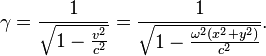
![]() . For the Lorentz factor in the SR we obtain the following:
. For the Lorentz factor in the SR we obtain the following:
With this in mind, the potentials and field strengths of the
acceleration field can be written as follows:
![]()
![]()
![]()
If we substitute ![]() ,
, ![]() ,
, ![]() and
and ![]() in (7), we can determine the
acceleration components of the particle and the acceleration amplitude:
in (7), we can determine the
acceleration components of the particle and the acceleration amplitude:
![]()
![]()
The acceleration is directed towards the center of rotation and
represents centripetal acceleration. Using now the classic vector description,
we have also for the time and coordinates of reference frame at the center of
rotation:
![]()
![]()
where ![]() and
and ![]() are two coordinates of the
cylindrical coordinate system,
are two coordinates of the
cylindrical coordinate system, ![]() is the vector from the center of
rotation to the particle,
is the vector from the center of
rotation to the particle, ![]() is the axial vector of the
differential of the rotation angle directed along the axis OZ.
is the axial vector of the
differential of the rotation angle directed along the axis OZ.
As we can see, in case of such a motion with acceleration the vector
product ![]() is not equal to zero, just as the
three-vector
is not equal to zero, just as the
three-vector ![]() of energy flux density of the acceleration field inside the particle.
of energy flux density of the acceleration field inside the particle.
System of particles
Due to interaction of a number of particles with each
other by means of various fields, including interaction at a distance without
direct contact, the acceleration field in the matter changes and is different
from the acceleration field of individual particles at the observation point. As a result, the density of the
4-force in the system of
particles is given by the strength and the solenoidal vector, which represent
the typical average characteristics of the matter motion. For example, in a
gravitationally bound system there is a radial gradient of the vector ![]() and if the system is moving or rotating,
there is a vector
and if the system is moving or rotating,
there is a vector ![]() From (5) there follows
the general expression for the density of 4-force with covariant index:
From (5) there follows
the general expression for the density of 4-force with covariant index:
![]()
where ![]() denotes a four-dimensional space-time
interval. For a stationary case, when the potentials of the acceleration field
are independent of time, under the assumption that
denotes a four-dimensional space-time
interval. For a stationary case, when the potentials of the acceleration field
are independent of time, under the assumption that ![]() wave equation (2) for the scalar potential
in the SR is transformed
into the equation:
wave equation (2) for the scalar potential
in the SR is transformed
into the equation:
![]()
The solution of this equation for
a fixed sphere with the particles randomly moving in it has the form: [12]
![]()
where  is the Lorentz factor for the velocities
 ![]() of the particles in the center of the
sphere, and due to the smallness of the argument the sine is expanded to the
second order terms. From the formula it follows that the average velocities of
the particles are maximal in the center and decrease when approaching the
surface of the sphere.
of the particles in the center of the
sphere, and due to the smallness of the argument the sine is expanded to the
second order terms. From the formula it follows that the average velocities of
the particles are maximal in the center and decrease when approaching the
surface of the sphere.
In such a system, the scalar
potential ![]() becomes the function of the radius, and the
vector potential
becomes the function of the radius, and the
vector potential ![]() and the solenoidal vector
and the solenoidal vector ![]() are equal to zero. The acceleration field
strength
are equal to zero. The acceleration field
strength ![]() is found with the help of (1). Then we can
calculate all the functions of the acceleration field, including the energy of
particles in this field and the energy of the acceleration field itself. [13] For cosmic bodies the main contribution to the four-acceleration
in the matter makes the gravitational force and the pressure field.
is found with the help of (1). Then we can
calculate all the functions of the acceleration field, including the energy of
particles in this field and the energy of the acceleration field itself. [13] For cosmic bodies the main contribution to the four-acceleration
in the matter makes the gravitational force and the pressure field.
At the same time the relativistic
rest energy of the system is automatically derived, taking into account the
motion of particles inside the sphere. For the system of particles with the
acceleration field, pressure field, gravitational and electromagnetic fields
the given approach allowed solving the 4/3 problem and showed where and in what
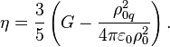
form the energy of the system is contained. The relation for the acceleration
field constant in this problem was found:
![]()
where ![]() is the electric
constant,
is the electric
constant, ![]() and
and ![]() are the total charge and mass of the
system.
are the total charge and mass of the
system.
The solution of the wave equation
for the acceleration field within the system results in temperature
distribution according to the formula: [12]
![]()
where ![]() is the temperature in the center,
is the temperature in the center, ![]() is the mass of the particle, for which the
mass of the proton is taken (for systems which are based on hydrogen or
nucleons in atomic nuclei),
is the mass of the particle, for which the
mass of the proton is taken (for systems which are based on hydrogen or
nucleons in atomic nuclei), ![]() is the mass of the system within the current
radius
is the mass of the system within the current
radius ![]() ,
, ![]() is the Boltzmann constant.
is the Boltzmann constant.
This dependence is well satisfied
for a variety of space objects, including gas clouds and Bok globules, the
Earth, the Sun and neutron stars.
In articles [14] [15]
the ratio of the field’s coefficients for the fields was specified as follows:
![]()
where ![]() is the
pressure field constant.
is the
pressure field constant.
If we introduce the parameter ![]() as the number
of nucleons per ionized gas particle, then the acceleration field constant is
expressed as follows:
as the number
of nucleons per ionized gas particle, then the acceleration field constant is
expressed as follows:
![]()
For the temperature inside the
cosmic bodies in the gravitational equilibrium model we find the dependence on
the current radius:
![]()
where ![]() is the mass of
one gas particle, which is taken as the unified atomic mass unit, and the
coefficients
is the mass of
one gas particle, which is taken as the unified atomic mass unit, and the
coefficients ![]() and
and ![]() are included
into the dependence of the mass density on the radius in the relation
are included
into the dependence of the mass density on the radius in the relation ![]()
Under the
assumption that the system’s typical particles have the mass ![]() , and that it is typical
particles that define the temperature and pressure, for the acceleration field
constant we obtain the following: [16]
, and that it is typical
particles that define the temperature and pressure, for the acceleration field
constant we obtain the following: [16]
The Lorentz
factor of the particles in the center of the system is also determined: [17]

The wave equation (3) for the
vector potential of the acceleration field was used to represent the relativistic
equation of the fluid’s motion in the form of the Navier–Stokes equations in hydrodynamics
and to describe the motion of the viscous compressible and charged
fluid. [10]
Taking into
account the acceleration field and pressure field, within the framework of the relativistic
uniform system, it is possible to refine the virial theorem, which in the relativistic form is written as follows: [18]
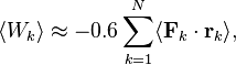
where the
value ![]() exceeds the kinetic energy of the
particles
exceeds the kinetic energy of the
particles ![]() by a factor equal to the Lorentz
factor
by a factor equal to the Lorentz
factor ![]() of the particles at the center
of the system. Under normal conditions we can assume that
of the particles at the center
of the system. Under normal conditions we can assume that ![]() , then we can see that in the
virial theorem the kinetic energy is related to the potential energy not by the
coefficient 0.5, but rather by the coefficient close to 0.6. The difference
from the classical case arises due to considering the pressure field and the
acceleration field of particles inside the system, while the derivative of the
virial scalar function
, then we can see that in the
virial theorem the kinetic energy is related to the potential energy not by the
coefficient 0.5, but rather by the coefficient close to 0.6. The difference
from the classical case arises due to considering the pressure field and the
acceleration field of particles inside the system, while the derivative of the
virial scalar function ![]() is not equal to zero and should
be considered as the material
derivative.
is not equal to zero and should
be considered as the material
derivative.
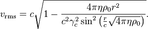
An analysis
of the integral theorem of generalized virial makes it possible to find, on the
basis of field theory, a formula for the root-mean-square speed of typical
particles of a system without using the notion of temperature: [19]
The integral
field
energy theorem for acceleration field in a curved
space-time is as follows:[11]

In the
relativistic uniform system, the scalar potential ![]() of the acceleration field is
related to the scalar potential
of the acceleration field is
related to the scalar potential ![]() of the pressure field: [20]
of the pressure field: [20]
![]()
The
relativistic expression for pressure is as follows:
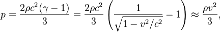
where ![]() is the mass density of moving
matter,
is the mass density of moving
matter, ![]() is the speed of light,
is the speed of light,  is the Lorentz factor. In the
limit of low velocities, this relationship turns into the standard formula of
the kinetic theory of gases.
is the Lorentz factor. In the
limit of low velocities, this relationship turns into the standard formula of
the kinetic theory of gases.
In [21]
it is shown how the acceleration field contributes to the mass of a physical
system. Similarly, the acceleration field contributes to the space-time metric,
both in the matter of the physical system and beyond it. [22]
The concept
of the acceleration field allows one to define in a covariant form in curved
space-time the generalized four-momentum, [23] the energy, momentum
and total four-momentum of a physical system taking into account particles and
fields, [5] and also the angular momentum
pseudotensor. [6]
Other approaches
Studying the Lorentz covariance of the 4-force, Friedman
and Scarr found incomplete covariance of the expression for the 4-force in the
form ![]() [24]
[24]
This led them to conclude that
the four-acceleration in special theory of relativity must be expressed
with the help of a certain antisymmetric tensor
![]() :
:
![]()
Based on the analysis of various
types of motion, they estimated the required values of components of tensor ![]() , thereby giving indirect definition to
this tensor.
, thereby giving indirect definition to
this tensor.
In contrast,
according to (5) the density of the 4-force is equal to ![]() and in (4)
and in (4) ![]() Thus, in a curved space-time, the
4-acceleration of an element of matter will be
Thus, in a curved space-time, the
4-acceleration of an element of matter will be
![]() . Taking this into account, the tensor
. Taking this into account, the tensor
![]() , up to a sign and a constant
factor, has the same meaning as the acceleration field tensor
, up to a sign and a constant
factor, has the same meaning as the acceleration field tensor ![]() .
.
Mashhoon and Muench considered transformation
of inertial reference frames, co-moving with the accelerated reference frame,
and obtained the relation: [25]
![]()
The tensor ![]() has the same properties as the acceleration field tensor
has the same properties as the acceleration field tensor ![]()
The use in general theory of relativity
The action function in the general relativity (GR) can be represented as
the sum of the four terms, which are responsible, respectively, for the
spacetime metric, the matter in the form of substance, the electromagnetic
field and the pressure field:
![]()
Additional terms can be included in the action function, if other fields
must be taken into account. The first, second and third terms of the action
have the standard form: [8]
![]()
![]()
![]()
where ![]() is the electromagnetic
four-potential.
is the electromagnetic
four-potential.
The term ![]() , which is responsible for the contribution of pressure into the action
function, is different in the works of different authors, depending on how the
pressure is related to the elastic energy and whether the pressure field is
considered to be a scalar field or a vector field. It should be noted that in
the GR, the gravitational field is included in the action function not
directly, but indirectly, by means of the metric tensor. In this case, as a
rule, the pressure field is considered to be a scalar field.
, which is responsible for the contribution of pressure into the action
function, is different in the works of different authors, depending on how the
pressure is related to the elastic energy and whether the pressure field is
considered to be a scalar field or a vector field. It should be noted that in
the GR, the gravitational field is included in the action function not
directly, but indirectly, by means of the metric tensor. In this case, as a
rule, the pressure field is considered to be a scalar field.
In contrast, in covariant theory of gravitation (CTG), the term ![]() associated with the acceleration
field is used instead of the term
associated with the acceleration
field is used instead of the term ![]() , and the action function can be written as follows: [4]
, and the action function can be written as follows: [4]
![]()
Here
![]()
![]()
where ![]() is the four-potential of the pressure
field,
is the four-potential of the pressure
field, ![]() is the coefficient of the
pressure field,
is the coefficient of the
pressure field, ![]() is the pressure field tensor,
is the pressure field tensor,
![]() .
.
In the case of rectilinear motion
of a rigid body without rotation, the following relations will hold: ![]() ,
, ![]() , and in the term
, and in the term ![]() the relation
the relation
![]() is obtained. In this particular case it is
clear that the term
is obtained. In this particular case it is
clear that the term ![]() differs from the term
differs from the term ![]() by an additional term associated with the
energy of the acceleration field.
by an additional term associated with the
energy of the acceleration field.
This is due to the fact that in the covariant theory of gravitation the
acceleration field is considered to be a vector field, whereas as in the
general relativity the acceleration field is actually used
as a scalar field that does not depend on the particles’ velocities. In both
theories, the acceleration field allows us to determine the contribution of the
rest energy of the particles into the total energy of the system of particles
and fields. However, the use of the acceleration field as a scalar field in the
general relativity does not agree in its form with the vector nature of the electromagnetic
field. Indeed, in the limiting case, when only the particles’ accelerations and
electromagnetic forces are taken into account, the acceleration must be
two-component, as is the case for the acceleration due to the action of the
two-component Lorentz force. But this is only possible in the case where the acceleration field
itself is a vector field. The situation can be improved if,
in addition to the gravitational field function, we ascribe to the metric
field ![]() in the general relativity the
function of the vector component of the acceleration field, but this makes the
equations of the theory even more complex and complicated.
in the general relativity the
function of the vector component of the acceleration field, but this makes the
equations of the theory even more complex and complicated.
It should be noted that in the general case of arbitrary
motion of the matter the relation ![]() is no longer satisfied and CTG does not
coincide any more with GR in the method of describing the rest energy of a
physical system. This means that in GR the motion of the matter is considered
in a simplified way, as rectilinear motion of a solid body, whereas in CTG the
use of the four-potential
is no longer satisfied and CTG does not
coincide any more with GR in the method of describing the rest energy of a
physical system. This means that in GR the motion of the matter is considered
in a simplified way, as rectilinear motion of a solid body, whereas in CTG the
use of the four-potential ![]() o f the acceleration field allows
us to take into account the internal motion of the matter in each selected
volume element. For example, when a particle moves round a circle, the
four-potential
o f the acceleration field allows
us to take into account the internal motion of the matter in each selected
volume element. For example, when a particle moves round a circle, the
four-potential ![]() of the particle’s matter will depend on the
location of this matter with respect to the circle line, since the velocity of
the particle’s matter depends on the radius of rotation.
of the particle’s matter will depend on the
location of this matter with respect to the circle line, since the velocity of
the particle’s matter depends on the radius of rotation.
See also
- General field
- Pressure field
- Dissipation
field
- Covariant theory of gravitation
- Metric theory of
relativity
- Acceleration tensor
- Acceleration stress-energy tensor
- Four-force
- Equation of
vector field
References
- 1.0 1.1 Fedosin S.G. The Concept of the General
Force Vector Field. OALib Journal, Vol. 3, pp. 1-15 (2016),
e2459. http://dx.doi.org/10.4236/oalib.1102459.
- Fedosin
S.G. Two components of the macroscopic general field. Reports in Advances
of Physical Sciences, Vol. 1, No. 2, 1750002, 9 pages (2017). http://dx.doi.org/10.1142/S2424942417500025.
- 3.0 3.1 Fedosin S.G. The procedure of finding
the stress-energy tensor and vector field equations of any form. Advanced Studies in Theoretical Physics, Vol.
8, No. 18, pp. 771-779 (2014). http://dx.doi.org/10.12988/astp.2014.47101.
- 4.0 4.1 4.2 Fedosin S.G. About the cosmological
constant, acceleration field, pressure field and energy. Jordan
Journal of Physics. Vol. 9, No. 1, pp. 1-30 (2016). http://dx.doi.org/10.5281/zenodo.889304.
- 5.0 5.1 Fedosin S.G. What should we understand by the four-momentum of
physical system? Physica Scripta, Vol.
99, No. 5, 055034 (2024). https://doi.org/10.1088/1402-4896/ad3b45.
- 6.0 6.1 Fedosin S.G. Lagrangian formalism in the theory of relativistic
vector fields. International Journal of Modern Physics A, Vol. 40, No. 02,
2450163 (2025). https://doi.org/10.1142/S0217751X2450163X.
- 7,0 7,1 7,2 Fedosin
S.G. Equations of Motion in the Theory of Relativistic Vector Fields.
International Letters of Chemistry, Physics and Astronomy, Vol. 83, pp.
12-30 (2019). https://doi.org/10.18052/www.scipress.com/ILCPA.83.12.
- 8.0 8.1
Fock, V.
A. (1964). "The Theory of Space, Time and Gravitation". Macmillan.
- Landau L.D., Lifshitz E.M. The Classical Theory
of Fields, (1951). Pergamon Press. ISBN 7-5062-4256-7.
- 10.0 10.1 Fedosin S.G. Four-Dimensional
Equation of Motion for Viscous Compressible and Charged Fluid with Regard
to the Acceleration Field, Pressure Field and Dissipation Field.
International Journal of Thermodynamics. Vol. 18, No. 1, pp. 13-24 (2015).
http://dx.doi.org/10.5541/ijot.5000034003.
- 11.0 11.1 Fedosin
S.G. The Integral Theorem of the Field Energy.
Gazi University Journal of Science. Vol. 32, No. 2, pp. 686-703 (2019). http://dx.doi.org/10.5281/zenodo.3252783.
- 12,0 12,1 Fedosin
S.G. The Integral Energy-Momentum
4-Vector and Analysis of 4/3 Problem Based on the Pressure Field and
Acceleration Field. American Journal of Modern Physics. Vol. 3, No. 4,
pp. 152-167 (2014). http://dx.doi.org/10.11648/j.ajmp.20140304.12.
- Fedosin S.G. Relativistic
Energy and Mass in the Weak Field Limit. Jordan Journal of Physics. Vol. 8, No. 1, pp. 1-16 (2015). http://dx.doi.org/10.5281/zenodo.889210.
- Fedosin S.G. Estimation
of the physical parameters of planets and stars in the gravitational
equilibrium model. Canadian Journal of Physics, Vol. 94, No. 4, pp.
370-379 (2016). http://dx.doi.org/10.1139/cjp-2015-0593.
- Fedosin S.G. The generalized Poynting theorem for the general field
and solution of the 4/3 problem. International Frontier Science Letters,
Vol. 14, pp. 19-40 (2019). https://doi.org/10.18052/www.scipress.com/IFSL.14.19.
- Fedosin S.G. The binding energy and the total energy of a
macroscopic body in the relativistic uniform model. Middle East Journal of
Science, Vol. 5, Issue 1, pp. 46-62 (2019). http://dx.doi.org/10.23884/mejs.2019.5.1.06.
- Fedosin S.G. Energy and metric gauging in the covariant theory of
gravitation. Aksaray University Journal of
Science and Engineering, Vol. 2, Issue 2, pp. 127-143 (2018). http://dx.doi.org/10.29002/asujse.433947.
- Fedosin S.G. The virial
theorem and the kinetic energy of particles of a macroscopic system in the
general field concept. Continuum Mechanics and Thermodynamics. Vol. 29,
Issue 2, pp. 361-371 (2017). https://dx.doi.org/10.1007/s00161-016-0536-8.
- Fedosin S.G. The integral theorem of
generalized virial in the relativistic uniform model. Continuum Mechanics and Thermodynamics, Vol.
31, Issue 3, pp. 627-638 (2019). https://dx.doi.org/10.1007/s00161-018-0715-x.
- Fedosin S.G. The potentials of the acceleration field and pressure field in
rotating relativistic uniform system. Continuum Mechanics and
Thermodynamics, Vol. 33, Issue 3, pp. 817-834 (2021). https://doi.org/10.1007/s00161-020-00960-7.
- Fedosin
S.G. The Mass Hierarchy in the Relativistic Uniform System. Bulletin of
Pure and Applied Sciences, Vol. 38 D (Physics), No. 2, pp. 73-80 (2019). http://dx.doi.org/10.5958/2320-3218.2019.00012.5.
- Fedosin
S.G. The relativistic uniform model: the metric of the covariant theory of
gravitation inside a body. St. Petersburg Polytechnical State University
Journal. Physics and Mathematics, Vol. 14, No. 3, pp.168-184 (2021). http://dx.doi.org/10.18721/JPM.14313.
- Fedosin
S.G. Generalized Four-momentum for Continuously Distributed Materials.
Gazi University Journal of Science, Vol. 37, Issue 3, pp. 1509-1538
(2024). https://doi.org/10.35378/gujs.1231793.
- Yaakov Friedman and
Tzvi Scarr. Covariant
Uniform Acceleration. Journal of Physics: Conference Series Vol. 437
(2013) 012009 doi:10.1088/1742-6596/437/1/012009.
- Bahram Mashhoon and Uwe Muench. Length measurement in
accelerated systems. Annalen der Physik. Vol.
11, Issue 7, P. 532–547, 2002.
External
links
·
Acceleration
field in Russian
Source:
http://sergf.ru/afen.htm