Physica Scripta, Vol. 99, No. 5,
055034 (2024). https://doi.org/10.1088/1402-4896/ad3b45
What should we understand by the four-momentum of physical system?
Sergey G. Fedosin
![]()
PO box 614088, Sviazeva str. 22-79, Perm, Perm Krai, Russia
E-mail:
fedosin@hotmail.com
It is shown that, in general, in curved spacetime, none of the known
definitions of four-momentum correspond to the definition, in which all the
system’s particles and fields, including fields outside matter, make an
explicit contribution to the four-momentum. This drawback can be eliminated
under the assumption that the primary representation of four-momentum is the
sum of two nonlocal four-vectors of the integral type with covariant indices.
The first of these four-vectors is the generalized four-momentum, found with
the help of Lagrangian density. The time component of the generalized
four-momentum, in theory of vector fields, is proportional to the particles’
energy in scalar field potentials, and the space component is related to vector
field potentials. The second four-vector is the four-momentum of fields
themselves, and its time component is related to the energy given by tensor
invariants. As a result, the system’s four-momentum is defined as a four-vector
with a covariant index. The standard approach makes it possible to find the
four-momentum in covariant form only for a free point particle. In contrast,
the obtained formulas for calculating the four-momentum components are applied
to a stationary and moving relativistic uniform system, consisting of many
particles. In this case, the main fields of the system under consideration are
taken into account, including the electromagnetic and gravitational fields, the
acceleration field and the pressure field. All these fields are considered
vector fields, which makes it possible to unambiguously determine the equations
of motion of the fields themselves and the equations of motion of matter in
these fields. The formalism used includes the principle of least action,
charged and neutral four-currents, corresponding four-potentials and field
tensors, which ensures unification and the possibility of combining fields into
a single interaction. Within the framework of the special theory of relativity,
it is shown that due to motion, the four-momentum of the system increases in
proportion to the Lorentz factor of the system’s center of momentum, while in
the matter of the system the sum of the energies of all fields is equal to
zero. The calculation of the integral vector’s components in the relativistic
uniform system shows that the so-called integral vector is not equal to
four-momentum and is not a four-vector at all, although it is conserved in a
closed system. Thus, in the theory of relativistic vector fields, the
four-momentum cannot be found with the help of an integral vector and
components of the system’s stress-energy tensor, in contrast to how it is
assumed in the general theory of relativity.
Keywords: generalized four-momentum; four-momentum of field; relativistic uniform system; integral vector.
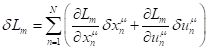
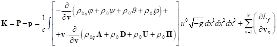
By the standard definition adopted in the theory of relativity, the
four-momentum of a physical system is a four-vector of the following form:
![]() , (1)
, (1)
where ![]() is energy,
is energy, ![]() is speed of
light, and
is speed of
light, and ![]() is three-dimensional relativistic
momentum of the system.
is three-dimensional relativistic
momentum of the system.
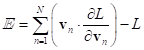
Definition (1) is widely used in mechanics for
equations of motion, where the derivative of four-momentum with respect to
proper time defines four-forces acting on a system. Both ![]() and
and ![]() are additive quantities, thus,
the energy is obtained by summing the energies contained in all the volume
elements of a system. The system momentum should be determined by vector
summation of the momenta of all volume elements, including those in which there
is no matter where there is only a field.
are additive quantities, thus,
the energy is obtained by summing the energies contained in all the volume
elements of a system. The system momentum should be determined by vector
summation of the momenta of all volume elements, including those in which there
is no matter where there is only a field.
The energy and momentum of a system,
which contains ![]() particles or individual elements of
continuously distributed matter, can be derived via Lagrangian formalism [1],
for which Lagrangian
particles or individual elements of
continuously distributed matter, can be derived via Lagrangian formalism [1],
for which Lagrangian ![]() is used as an integral over an
infinite moving volume:
is used as an integral over an
infinite moving volume:
![]() , (2)
, (2)
![]() , (4)
, (4)
here ![]() is Lagrangian density as volumetric density of
Lagrange function,
is Lagrangian density as volumetric density of
Lagrange function, ![]() is product of differentials of space
coordinates,
is product of differentials of space
coordinates, ![]() is determinant of metric tensor
is determinant of metric tensor ![]() ,
, ![]() is velocity of matter particle with
the current number
is velocity of matter particle with
the current number ![]() , and
, and ![]() is three-dimensional momentum of one
volume element of the system.
is three-dimensional momentum of one
volume element of the system.
Substituting (3) and (4) in (1) allows us to find ![]() . However, such a definition of four-momentum is
unsatisfactory in the sense that it is not a direct consequence of Lagrangian
four-dimensional formalism for four-vectors and four-tensors. As far as we
know,
. However, such a definition of four-momentum is
unsatisfactory in the sense that it is not a direct consequence of Lagrangian
four-dimensional formalism for four-vectors and four-tensors. As far as we
know, ![]() as a four-vector is not expressed in
a covariant form either with the help of Lagrangian
as a four-vector is not expressed in
a covariant form either with the help of Lagrangian ![]() or with the
help of Lagrangian density
or with the
help of Lagrangian density ![]() , the four-momentum
, the four-momentum ![]() is simply constructed manually using
formula (1). Instead, in [2], we can find a covariant expression of
four-momentum but only for one free particle, on which no external forces are
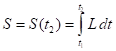
acting. In this case, the definition of the action function
is simply constructed manually using
formula (1). Instead, in [2], we can find a covariant expression of
four-momentum but only for one free particle, on which no external forces are
acting. In this case, the definition of the action function ![]() with a variable upper limit of
integration is used:
with a variable upper limit of
integration is used:
 .
(5)
.
(5)
![]() . (6)
. (6)
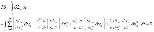
The characteristic feature of (5) is that the upper limit in the time
integral for the action function is not fixed, in contrast to the lower limit.
In addition, a particle must move with zero four-acceleration along a certain
true trajectory according to its equation of motion. Under such conditions, the
variation in the particle’s location at the initial time point is equal to
zero, ![]() ; however, the variation
; however, the variation ![]() at time point
at time point ![]() is not equal to
zero. According to (6), the four-momentum
is not equal to
zero. According to (6), the four-momentum ![]() of a single
particle turns out to be a four-vector with a covariant index, in contrast to
(1), where the four-momentum
of a single
particle turns out to be a four-vector with a covariant index, in contrast to
(1), where the four-momentum ![]() of a system of
particles is presented as a four-vector with a contravariant index.
of a system of
particles is presented as a four-vector with a contravariant index.
In the flat Minkowski spacetime, the difference between a four-vector
with a covariant index and the same four-vector with a contravariant index
consists only of the fact that their space components have opposite signs. In
curved spacetime, the difference is more significant since to turn to a
contravariant form, the four-vector with a covariant index must be multiplied
by the metric tensor. In this case, it is more convenient to write equations
for the particle through ![]() (6) rather than
through
(6) rather than
through ![]() , since then the metric tensor is not required. This can significantly simplify the solution of the
equation of motion, since the metric tensor may not be known in advance.
, since then the metric tensor is not required. This can significantly simplify the solution of the
equation of motion, since the metric tensor may not be known in advance.
In a system, consisting of many closely interacting particles, different
forces are acting and the particles acquire four-accelerations. This violates
conditions, under which definition (6) is valid, so that the summation of
four-momenta of individual particles may not provide the total four-momentum ![]() of the system.
Thus, for continuously distributed matter, another covariant expression is
required for both the four-momentum of a single particle and the four-momentum
of the entire system.
of the system.
Thus, for continuously distributed matter, another covariant expression is
required for both the four-momentum of a single particle and the four-momentum
of the entire system.
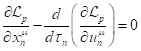
According to [3], the covariant four-dimensional Euler–Lagrange equation should have the following form:
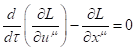 , (7)
, (7)
where ![]() is four-velocity,
is four-velocity, ![]() is proper time of a particle, and
is proper time of a particle, and ![]() is four-position that determines
location of the particle.
is four-position that determines
location of the particle.
The equation (7) is the result of variation of the Lagrange function ![]() in the principle of least action and
represents the equation of particle motion. To apply (7), it is necessary to
know the dependence
in the principle of least action and
represents the equation of particle motion. To apply (7), it is necessary to
know the dependence ![]() on the values
on the values ![]() and
and ![]() of each individual particle of the system, which turns out to be
difficult with a large number of particles.
of each individual particle of the system, which turns out to be
difficult with a large number of particles.
The quantity ![]() in (7) can be
interpreted as the four-momentum of an arbitrary particle of a physical system,
the quantity
in (7) can be
interpreted as the four-momentum of an arbitrary particle of a physical system,
the quantity ![]() can be considered as a four-force
acting on the particle, and the total four-momentum must be obtained by summing
individual quantities
can be considered as a four-force
acting on the particle, and the total four-momentum must be obtained by summing
individual quantities ![]() over all the system’s particles. However, here, a difficulty arises
with respect to contributing to four-momentum from fields outside the matter’s
limits, which are characterized in Lagrangian form with the help of volume integrals of tensor invariants. The expression
of volume integrals of the tensor invariants in terms of the four-velocity of
particles is by itself a rather complicated and nontrivial task.
over all the system’s particles. However, here, a difficulty arises
with respect to contributing to four-momentum from fields outside the matter’s
limits, which are characterized in Lagrangian form with the help of volume integrals of tensor invariants. The expression
of volume integrals of the tensor invariants in terms of the four-velocity of
particles is by itself a rather complicated and nontrivial task.
There is a completely different approach to determining the system’s
four-momentum, associated with the general theory of relativity. Therefore, in
[2] we can find the following expression:
![]() , (8)
, (8)
where the time components of the stress-energy tensor
of matter and nongravitational fields are denoted by ![]() , and the time components of the gravitational field pseudotensor are
denoted by
, and the time components of the gravitational field pseudotensor are
denoted by ![]() .
.
It is argued that quantity ![]() is simply the four-momentum
is simply the four-momentum ![]() of a physical system, taking into
account the contribution from gravitational field, while in a closed system
of a physical system, taking into
account the contribution from gravitational field, while in a closed system ![]() is conserved. In this regard, we
should note that to obtain
is conserved. In this regard, we
should note that to obtain ![]() , it is necessary to proceed from the
equation of motion in the form
, it is necessary to proceed from the
equation of motion in the form ![]() . Then, such a gravitational field pseudotensor
. Then, such a gravitational field pseudotensor ![]() is introduced into this equation to transform from a
covariant derivative to a partial derivative. The equation of motion takes the
form
is introduced into this equation to transform from a
covariant derivative to a partial derivative. The equation of motion takes the
form ![]() , after which it is integrated over volume, resulting in (8).
, after which it is integrated over volume, resulting in (8).
The drawback of this approach is the
lack of evidence that ![]() is truly the system’s
four-momentum. Expressions (3) and (4) for the
energy and momentum do not automatically follow from (8), and it is difficult
to determine whether (8) is associated with (6) or with
is truly the system’s
four-momentum. Expressions (3) and (4) for the
energy and momentum do not automatically follow from (8), and it is difficult
to determine whether (8) is associated with (6) or with ![]() in
(7). Moreover, according to [4], there are many different gravitational field
pseudotensors, which give different expressions for
in
(7). Moreover, according to [4], there are many different gravitational field
pseudotensors, which give different expressions for ![]() ; therefore, there is no guarantee that at least in one case the
equality
; therefore, there is no guarantee that at least in one case the
equality ![]() would hold. In addition, in [5],
the correspondence principle was not fulfilled in the general theory of
relativity, and the inertial mass in general case within the limits of weak
fields and low velocities was not included in the corresponding expression in
Newton’s theory. According to [6], the same holds
true for the energy, momentum and angular momentum of a system.
would hold. In addition, in [5],
the correspondence principle was not fulfilled in the general theory of
relativity, and the inertial mass in general case within the limits of weak
fields and low velocities was not included in the corresponding expression in
Newton’s theory. According to [6], the same holds
true for the energy, momentum and angular momentum of a system.
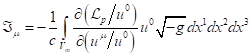
In [7], a comparison was made
between the vector ![]() and the integral vector, obtained
by the following formula:
and the integral vector, obtained
by the following formula:
![]() .
(9)
.
(9)
Expression (9) for the integral
vector ![]() is valid for the case of weak
fields and low velocities, when the covariant derivative
is valid for the case of weak
fields and low velocities, when the covariant derivative ![]() in the equation of motion
in the equation of motion ![]() can be replaced with the partial
derivative
can be replaced with the partial
derivative ![]() with a small error. The quantity
with a small error. The quantity ![]() with mixed indexes in (9) defines
the time components of the system’s stress-energy tensor, while the
gravitational field is considered a vector field within the framework of the
covariant theory of gravitation [8]. Analysis of the vector
with mixed indexes in (9) defines
the time components of the system’s stress-energy tensor, while the
gravitational field is considered a vector field within the framework of the
covariant theory of gravitation [8]. Analysis of the vector ![]() shows that its time component is
related to the sum of energies of all the system’s fields, and the space
component is related to the vector sum of field energy flux vectors. If the
four-momentum
shows that its time component is
related to the sum of energies of all the system’s fields, and the space
component is related to the vector sum of field energy flux vectors. If the
four-momentum ![]() defines the energy and momentum
of the system’s particles and fields, then the vector
defines the energy and momentum
of the system’s particles and fields, then the vector ![]() defines only the energies and
fields’ energy fluxes.
defines only the energies and
fields’ energy fluxes.
According to the method of its
construction, the integral vector ![]() is not a four-vector and can be
considered a four-dimensional pseudovector. For the vector
is not a four-vector and can be
considered a four-dimensional pseudovector. For the vector ![]() in (8), this vector has the property
that does not allow us to simultaneously fulfill two conditions for a closed
system [9]:
in (8), this vector has the property
that does not allow us to simultaneously fulfill two conditions for a closed
system [9]:
1) Conservation over time of the sum
of all types of energy, including gravitational energy given by the
pseudotensor; 2) independence of the sum of all types of energy at a given time
point from the choice of reference frame. As a result, in [10] vectors such as ![]() in the general theory of relativity
are considered not as four-vectors but rather as pseudovectors that cannot
define four-momentum
in the general theory of relativity
are considered not as four-vectors but rather as pseudovectors that cannot
define four-momentum ![]() .
.
The purpose of this work is to
derive a covariant formula for the system’s four-momentum, which is valid for
curved spacetime and for continuously distributed matter. Considering the
latter circumstance leads to the fact that instead of Lagrangian ![]() , the Lagrangian density
, the Lagrangian density ![]() takes the first place in
calculations. Our analysis includes the four most
common fields, electromagnetic and gravitational fields, acceleration field
[11], and pressure field [12], which are considered vector fields. The Lagrangian formalism we use allows us to consider all these fields
as components of a single general field [13-15], while the forces acting in the
system from each field have the same form, similar to the Lorentz force.
takes the first place in
calculations. Our analysis includes the four most
common fields, electromagnetic and gravitational fields, acceleration field
[11], and pressure field [12], which are considered vector fields. The Lagrangian formalism we use allows us to consider all these fields
as components of a single general field [13-15], while the forces acting in the
system from each field have the same form, similar to the Lorentz force.
As we will show below, the derived
formula for four-momentum will differ from the well-known standard definitions.
In addition, by direct calculation of the integral vector ![]() , we will show its difference from the
four-momentum of the moving physical system.
, we will show its difference from the
four-momentum of the moving physical system.
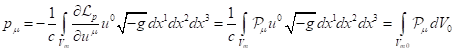
Appendix A briefly
describes two ways of representing the four-momentum ![]() of a physical system.
In the first of these methods, it is necessary to calculate the energy and
momentum of the system, and in the second method, the four-momentum
of a physical system.
In the first of these methods, it is necessary to calculate the energy and
momentum of the system, and in the second method, the four-momentum ![]() is represented as the
sum of two nonlocal integral vectors in the form
is represented as the
sum of two nonlocal integral vectors in the form ![]() . Appendix B provides details of calculations in relations (119-122).
Appendix C provides a list of symbols used.
. Appendix B provides details of calculations in relations (119-122).
Appendix C provides a list of symbols used.
2. Methods
Before considering the four-momentum of a physical system, it is
necessary to define the generalized four-momentum, which is the main part of the four-momentum.
To calculate the generalized
four-momentum, we will proceed from the Lagrangian formalism for continuously
distributed matter in four-dimensional form. In the general case, the
Lagrangian density depends on coordinate time ![]() , on charge four-currents
, on charge four-currents ![]() and mass four-current
and mass four-current ![]() , on four-potentials and field
tensors at each point in the field, including inside the particles, as well as
on the metric tensor
, on four-potentials and field
tensors at each point in the field, including inside the particles, as well as
on the metric tensor ![]() and the scalar curvature
and the scalar curvature ![]() :
:
![]() , (10)
, (10)
where ![]() specifies the observation point at which a
typical particle with number
specifies the observation point at which a
typical particle with number ![]() is located at a given moment in time, and
is located at a given moment in time, and ![]() is a four-velocity of the typical particle at
this point.
is a four-velocity of the typical particle at
this point.
In (10), ![]() denote the four-potentials of
electromagnetic and gravitational fields, acceleration field and pressure
field, respectively, and
denote the four-potentials of
electromagnetic and gravitational fields, acceleration field and pressure
field, respectively, and ![]() are tensors of these fields.
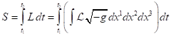
Considering (2), the action function within the time interval
are tensors of these fields.
Considering (2), the action function within the time interval ![]() with fixed integration limits is
equal to:
with fixed integration limits is
equal to:
 .
(11)
.
(11)
After substituting (10) into (11),
we can vary the action function and obtain equations for each field, equation
for metric and equation of motion of particles of
matter [11], [16]. In addition, we obtain the
four-dimensional Euler–Lagrange equation for each typical particle [17]:
 . (12)
The quantity ![]() in (12) represents the part of
the Lagrangian density
in (12) represents the part of
the Lagrangian density ![]() , which contains mass four-current
, which contains mass four-current ![]() and charge four-current
and charge four-current ![]() since only four-currents can
depend directly on the four-position
since only four-currents can
depend directly on the four-position ![]() and on the four-velocity
and on the four-velocity ![]() of particles. All the other
quantities in the Lagrangian, including four-potentials, field tensors and
metric tensor, become functions of
of particles. All the other
quantities in the Lagrangian, including four-potentials, field tensors and
metric tensor, become functions of ![]() and
and ![]() only after solving corresponding
equations; therefore, they are not differentiated in (12), behaving as
constants.
only after solving corresponding
equations; therefore, they are not differentiated in (12), behaving as
constants.
Indeed, the equation of any field is obtained only after varying the
Lagrangian in the principle of least action on the four-potential of the
corresponding field. This equation gives a relation between the four-current
generating the field and the field tensor. Considering the expression of the
field tensor in terms of the four-potential, the field equation can also be
represented as a relation between the four-current and four-potential. When
varying, it is assumed that the field tensor directly depends only on the
four-potential and its derivatives. As an example, we can consider Maxwell's
equations for the electromagnetic field, the solutions of which give either the
electromagnetic tensor or the four-potential as a function of the four-current
with a known dependence on time, coordinates and velocities.
On the other hand, in (10) all quantities in the large bracket are
assumed to be independent of each other from the point of view of the procedure
for varying these quantities. At the same time, ![]() and
and ![]() appear in the Lagrangian not directly, but
indirectly, since the four-currents
appear in the Lagrangian not directly, but
indirectly, since the four-currents ![]() and
and ![]() depend on them. As a result, variations of
four-currents in the Lagrangian are reduced to variations from
depend on them. As a result, variations of
four-currents in the Lagrangian are reduced to variations from ![]() [8], [11], [18].
[8], [11], [18].
The characteristic feature of (12) is that it is valid for a small
interval ![]() when the time components
when the time components ![]() of the particles’ four-velocities can be
assumed to be constant. If the interval
of the particles’ four-velocities can be
assumed to be constant. If the interval ![]() cannot be considered small, it should be
divided into small time intervals, and at each of these intervals, we should
perform synchronous variation of the action function and specify averaged
constant time components
cannot be considered small, it should be
divided into small time intervals, and at each of these intervals, we should
perform synchronous variation of the action function and specify averaged
constant time components ![]() of the particles’ four-velocities. On the other hand, equation (12)
can be understood as an equation for typical particles of a system; in this
case, the constancy
of the particles’ four-velocities. On the other hand, equation (12)
can be understood as an equation for typical particles of a system; in this
case, the constancy ![]() for each of the particles is
obtained automatically as a result of averaging the parameters of the particles at each point of the system.
for each of the particles is
obtained automatically as a result of averaging the parameters of the particles at each point of the system.
In contrast to the equation of motion (7), in
which the four-force ![]() appears, the equation of motion (12) is
written for the rate of change of the density of the four-momentum and for the density of the four-force
appears, the equation of motion (12) is
written for the rate of change of the density of the four-momentum and for the density of the four-force ![]() acting in a unit element of the volume in which a typical particle is
located.
acting in a unit element of the volume in which a typical particle is
located.
3. Results
3.1. Generalized four-momentum
With the help of (12) in [17], the
generalized four-momentum was determined:
 . (13)
In (13) ![]() is the volume density
of the generalized four-momentum, which is presented in (12),
is the volume density
of the generalized four-momentum, which is presented in (12), ![]() defines the time component of the
particles’ four-velocity at each integration point over the volume
defines the time component of the
particles’ four-velocity at each integration point over the volume ![]() , occupied by matter. In addition, a relation from [2] is
used:
, occupied by matter. In addition, a relation from [2] is
used:
![]() , (14)
, (14)
where ![]() is the differential of invariant volume of any of the particles of continuously distributed matter,
calculated in the particle’s comoving reference frame.
is the differential of invariant volume of any of the particles of continuously distributed matter,
calculated in the particle’s comoving reference frame.
In a closed system, the four-vector ![]() is conserved and represents the generalized four-momentum of all the system’s particles.
is conserved and represents the generalized four-momentum of all the system’s particles.
In addition to ![]() in (13), the following four-dimensional quantity can be determined:
in (13), the following four-dimensional quantity can be determined:
 . (15)
The quantity ![]() is not a four-vector, but under
the condition of constancy of
is not a four-vector, but under
the condition of constancy of ![]() , expression (15) becomes expression (13) for
, expression (15) becomes expression (13) for ![]() . As shown in [17], for purely vector
fields, part of the Lagrangian density
. As shown in [17], for purely vector
fields, part of the Lagrangian density ![]() is such that the space components
of
is such that the space components
of ![]() and
and ![]() coincide with each other and, up
to a sign, give the particles’ relativistic momentum
coincide with each other and, up
to a sign, give the particles’ relativistic momentum ![]() , which is part of (4). To calculate
, which is part of (4). To calculate ![]() , instead of entire Lagrangian
, instead of entire Lagrangian ![]() , we need to substitute into (4) its
part
, we need to substitute into (4) its
part ![]() , associated with four-currents.
, associated with four-currents.
3.2. Field energy in matter
By solving
equations for fields and metric inside matter, we can express four-potentials,
field tensors, metric tensor and scalar curvature in terms of four-positions ![]() and four-velocities
and four-velocities ![]() of system particles. In this case, inside the
matter the Lagrangian density (10) takes the form
of system particles. In this case, inside the
matter the Lagrangian density (10) takes the form ![]() . Using (2) and (14), we find:
. Using (2) and (14), we find:
![]() .
(16)
.
(16)
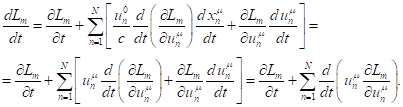
Expression
(17) represents the derivative of the Lagrange function ![]() with respect to coordinate time
with respect to coordinate time ![]() . This derivative is written as a
derivative of a complex function under the assumption that
. This derivative is written as a
derivative of a complex function under the assumption that ![]() and
and ![]() are functions of time
are functions of time ![]() .
.
The isochronous variation ![]() of the Lagrange function
of the Lagrange function![]() , taking into account standard equality to zero of variation of coordinate
time
, taking into account standard equality to zero of variation of coordinate
time ![]() , is expressed in terms of
variations
, is expressed in terms of
variations ![]() and
and ![]() :
:
 . (18)
Since ![]() ,
, ![]() , we obtain:
, we obtain:
 (19)
(19)
In (19), variation of the product of
two functions was used in the form:
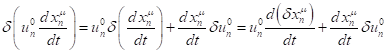 .
.
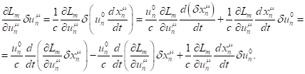
Substitution ![]() from (19) to (18) gives the
following:
from (19) to (18) gives the
following:
 (20)
(20)
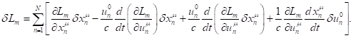
We substitute ![]() into (11) instead of
into (11) instead of ![]() , find the action variation and, in view of (20), equate it to zero:
, find the action variation and, in view of (20), equate it to zero:
(21)
As in [17], we assume that in the volume of each particle the time components ![]() of the particles’ four-velocity
are constant during the action variation, so that
of the particles’ four-velocity
are constant during the action variation, so that ![]() and the last term in (21) is equal to zero. Then for the next-to-last term in
(21), we can write the following:
and the last term in (21) is equal to zero. Then for the next-to-last term in
(21), we can write the following:
 (22))
(22))
The equality to
zero in (22) follows from the fact that variations ![]() at the time points
at the time points ![]() and
and ![]() vanish
according to the conditions of variation. In (21) the first two terms remain,
the difference between which must be equal to zero, as a consequence of
vanish
according to the conditions of variation. In (21) the first two terms remain,
the difference between which must be equal to zero, as a consequence of ![]() in the principle of least action.
This gives the following:
in the principle of least action.
This gives the following:
 .
(23)
.
(23)
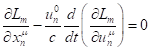
The equation (23) corresponds to (7) with the
difference that the Lagrangian ![]() inside matter is used instead of
inside matter is used instead of ![]() .
.
Let us express ![]() from (23) and substitute it into (17), taking
into account the relation
from (23) and substitute it into (17), taking
into account the relation ![]() :
:
 (24)
(24)
Relation (24) can be written as
follows: ![]() , where
, where
 . (25)
If the Lagrangian ![]() inside matter does not depend on
time, then
inside matter does not depend on
time, then ![]() and will be
and will be ![]() ,
, ![]() ; that is, the quantity
; that is, the quantity ![]() will be constant in time and will
not depend on coordinates.
will be constant in time and will
not depend on coordinates.
From the sum
over particles in (25) we can pass on to the integral over volume of
continuously distributed matter, expressing the Lagrangian ![]() through the
Lagrangian density
through the
Lagrangian density ![]() using (16):
using (16):
In the relation presented above, the
sum  was replaced by a sum
  in which the integral
 ![]() is taken only over the volume of
one particle with number
is taken only over the volume of
one particle with number ![]() . This is possible because the derivative
. This is possible because the derivative  is taken only with respect to the
four-velocity
is taken only with respect to the
four-velocity ![]() of the particle with number
of the particle with number ![]() . Therefore, the integral
. Therefore, the integral ![]() over the volume of all other
particles of the system does not depend on the four-velocity
over the volume of all other
particles of the system does not depend on the four-velocity ![]() of the particle with number
of the particle with number ![]() and the derivative for all other particles becomes
equal to zero.
and the derivative for all other particles becomes
equal to zero.
After this, the four-velocity ![]() is entered under the sign of
the integral
is entered under the sign of
the integral ![]() over the invariant volume
over the invariant volume ![]() of one particle, taking into
account that
of one particle, taking into
account that ![]() is constant within the volume of
this particle. In the integral
is constant within the volume of
this particle. In the integral ![]() , the volume element
, the volume element ![]() does not depend on the
four-velocity
does not depend on the
four-velocity ![]() , so the partial derivative
, so the partial derivative ![]() is also introduced inside the
integral and acts there on
is also introduced inside the
integral and acts there on ![]() .
.
Next, the sum  in the expression for
 ![]() is converted into an integral
is converted into an integral ![]() over the volume of all particles.
over the volume of all particles.
Subsequent use of expression (14)
for the volume element gives:
 (26)
(26)
In (21), we assumed that the time
components ![]() of the four-velocity of particles
are constant during the action variation. In this regard, the time component
of the four-velocity of particles
are constant during the action variation. In this regard, the time component ![]() of the four-velocity in (26) is
also considered as a constant value when calculating the derivative
of the four-velocity in (26) is
also considered as a constant value when calculating the derivative ![]() .
.
By comparing (25) and (3), we can
see that the quantity ![]() has dimension of energy. To
better understand the meaning of
has dimension of energy. To
better understand the meaning of ![]() , we use the Lagrangian density expression for four vector fields [11],
[19], which consists of two parts:
, we use the Lagrangian density expression for four vector fields [11],
[19], which consists of two parts:
![]()
(28)
where ![]() is four-potential of electromagnetic field, defined by scalar potential
is four-potential of electromagnetic field, defined by scalar potential ![]() and vector potential
and vector potential ![]() of this field,
of this field,
![]() is charge four-current,
is charge four-current,
![]() is charge density in particle’s
comoving reference frame,
is charge density in particle’s
comoving reference frame,
![]() is four-velocity of a point particle,
is four-velocity of a point particle,
![]() is four-potential of
gravitational field, described with the help of scalar potential
is four-potential of
gravitational field, described with the help of scalar potential ![]() and vector potential
and vector potential ![]() within the framework of covariant theory of
gravitation,
within the framework of covariant theory of
gravitation,
![]() is mass four-current,
is mass four-current,
![]() is mass density in particle’s
comoving reference frame,
is mass density in particle’s
comoving reference frame,
![]() is four-potential of
acceleration field, where
is four-potential of
acceleration field, where ![]() and
and ![]() denote scalar and vector
potentials, respectively,
denote scalar and vector
potentials, respectively,
![]() is four-potential of
pressure field, consisting of scalar potential
is four-potential of
pressure field, consisting of scalar potential ![]() and vector potential
and vector potential ![]() ;
;
![]() is magnetic constant,
is magnetic constant,
![]() is electromagnetic tensor,
is electromagnetic tensor,
![]() is gravitational constant,
is gravitational constant,
![]() is gravitational tensor,
is gravitational tensor,
![]() is acceleration field coefficient,
is acceleration field coefficient,
![]() is acceleration tensor, calculated as
four-curl of four-potential of acceleration field,
is acceleration tensor, calculated as
four-curl of four-potential of acceleration field,
![]() is pressure field coefficient,
is pressure field coefficient,
![]() is pressure field tensor,
is pressure field tensor,
![]() , where
, where ![]() is a certain coefficient of the order of unity
to be determined,
is a certain coefficient of the order of unity
to be determined,
![]() is scalar curvature,
is scalar curvature,
![]() is cosmological constant.
is cosmological constant.
The components ![]() and
and ![]() of Lagrangian density
of Lagrangian density ![]() in (27-28) have the remarkable
feature that all fields, be it an electromagnetic field or a pressure field,
are expressed in the same form, that is, through their own four-potentials and
through the corresponding tensors. It is well known that the electromagnetic
field in this form completely describes electromagnetic phenomena, including
all phenomena in curved spacetime with known metric, and taking into account
quantization it describes phenomena in the microworld within the framework of
quantum electrodynamics with very high accuracy. The same should be expected
for other fields in (27-28).
in (27-28) have the remarkable
feature that all fields, be it an electromagnetic field or a pressure field,
are expressed in the same form, that is, through their own four-potentials and
through the corresponding tensors. It is well known that the electromagnetic
field in this form completely describes electromagnetic phenomena, including
all phenomena in curved spacetime with known metric, and taking into account
quantization it describes phenomena in the microworld within the framework of
quantum electrodynamics with very high accuracy. The same should be expected
for other fields in (27-28).
For example, in [19] it was shown
that the covariant equation of particle motion in electromagnetic and
gravitational fields, in the acceleration field, in the pressure field and in
the dissipation field, after simplification within the framework of the special
theory of relativity, exactly transforms into the phenomenological
Navier-Stokes equation in hydrodynamics.
As another example, let us take the
pressure field, which is still, even in models of stars at high pressures,
treated as a scalar field. However, considering the pressure field as a vector
field significantly increases the accuracy of the results obtained, since in
this case a new degree of freedom appears in the form of a vector potential of
the pressure field, which is responsible for vector effects depending on the
particle velocity. Thus, we can consider our choice of the Lagrangian in
(27-28) to be completely justified.
Outside the matter, part of the
Lagrangian density ![]() vanishes since four-currents
vanishes since four-currents ![]() and
and ![]() are equal to zero, and in
are equal to zero, and in ![]() , tensors of acceleration field and
pressure field, which are present only inside the matter, vanish. When
calculating energy and momentum in the matter, we can neglect the last two
terms in
, tensors of acceleration field and
pressure field, which are present only inside the matter, vanish. When
calculating energy and momentum in the matter, we can neglect the last two
terms in ![]() for two reasons. First, the scalar curvature
for two reasons. First, the scalar curvature ![]() is a function of the metric
tensor and its derivatives, and it does not directly contain four-velocity;
thus,
is a function of the metric
tensor and its derivatives, and it does not directly contain four-velocity;
thus, ![]() . Second, we use such energy gauge and equation for metric, that
difference
. Second, we use such energy gauge and equation for metric, that
difference ![]() in (28) vanishes [11], [20].
in (28) vanishes [11], [20].
The Lagrangian density ![]() is similar to the Lagrangian
density
is similar to the Lagrangian
density ![]() in (27), but is calculated only
inside the matter. We take into account that four-velocity
in (27), but is calculated only
inside the matter. We take into account that four-velocity ![]() is present only in
is present only in ![]() (27), where it is part of four-currents. Consequently,
(27), where it is part of four-currents. Consequently,
![]() . (29)
. (29)
In view of (27-29), we find the
quantity ![]() in (26):
in (26):
 .
(30)
.
(30)
In (30), integration is performed
over the volume occupied by the matter. Hence, the energy ![]() is expressed exclusively in terms
of field tensors and is conserved if the Lagrangian inside the matter does not
directly depend on time. The last condition is satisfied for Lagrangian (27) so
that in a closed system the field energy, associated with tensor invariants,
must be conserved.
is expressed exclusively in terms
of field tensors and is conserved if the Lagrangian inside the matter does not
directly depend on time. The last condition is satisfied for Lagrangian (27) so
that in a closed system the field energy, associated with tensor invariants,
must be conserved.
3.3. Energy and momentum of a system
In (27-28), the Lagrangian density is presented in the form ![]() , where
, where ![]() depends on four-potentials and four-currents,
and
depends on four-potentials and four-currents,
and ![]() contains fields’ tensor invariants.
Additionally, Lagrangian
contains fields’ tensor invariants.
Additionally, Lagrangian ![]() is divided into two parts, one of which
is divided into two parts, one of which ![]() is associated with particles, and the other
is associated with particles, and the other ![]() is associated with fields.
is associated with fields.
In view of (2), we can write: ![]() . To calculate derivative
. To calculate derivative ![]() in expression for energy (3), it is necessary
to express
in expression for energy (3), it is necessary
to express ![]() of the Lagrangian in terms of the integral
over invariant volumes of particles. In view of (14), we find:
of the Lagrangian in terms of the integral
over invariant volumes of particles. In view of (14), we find:
![]() ,
, ![]() ,
,
In the sum presented above, the integral ![]() over the volume of all particles was replaced
by the integral
over the volume of all particles was replaced
by the integral  over the volume of a particle with respect to which the partial
derivative
over the volume of a particle with respect to which the partial
derivative ![]() is taken, the result does not change. After this,
is taken, the result does not change. After this, ![]() and
and ![]() are entered under the integral sign of , then the sum
are entered under the integral sign of , then the sum ![]() of the integrals over all particles turns into an integral over the
volume of all particles, giving
of the integrals over all particles turns into an integral over the
volume of all particles, giving  . Taking this into account, from (3)
we find:
. Taking this into account, from (3)
we find:
(31)
Taking into account the definitions ![]() and
and ![]() , we express both the charge four-current
, we express both the charge four-current
![]() and the mass four-current
and the mass four-current ![]() in the following form:
in the following form:
 .
.
 .
(32)
.
(32)
The products of the electromagnetic four-potential by charge
four-current and of the gravitational four-potential by mass four-current in
view of (32) can be represented as follows:
![]() ,
, ![]() . (33)
. (33)
Similarly, we can write for
acceleration field and for pressure field:
![]() ,
, ![]() . (34)
. (34)
Using expressions (33-34), in (27) ![]() is expressed in terms of velocity
is expressed in terms of velocity ![]() of motion of a matter element or a typical
particle:
of motion of a matter element or a typical
particle:
![]() . (35)
. (35)
We substitute ![]() from (35) and
from (35) and ![]() from (28) into (31) and obtain the following
expression for the energy of the system:
from (28) into (31) and obtain the following
expression for the energy of the system:
(36)
It was assumed in (36) that, in the
general case, the average field potentials in the particles’ volume, mass
density ![]() and charge density
and charge density ![]() of the particles can depend on
velocity
of the particles can depend on
velocity ![]() of these particles. When
substituting
of these particles. When
substituting ![]() , the energy gauge condition was used, according to which the difference
, the energy gauge condition was used, according to which the difference
![]() in (28) was taken to be equal to
zero [11], [20].
in (28) was taken to be equal to
zero [11], [20].
For momentum (4), in view of (2),
(35) and expression ![]() , we can write:
, we can write:
(37)
In (37), the derivative ![]() of the integral
of the integral ![]() over the volume of all particles was replaced
by the derivative
over the volume of all particles was replaced
by the derivative ![]() of the integral over the invariant volume of the particle with
number
of the integral over the invariant volume of the particle with
number ![]() , which has velocity
, which has velocity ![]() .
.
After this, the derivative ![]() was introduced under the sign of this integral
and the indices
was introduced under the sign of this integral
and the indices ![]() inside the integral were removed.
inside the integral were removed.
3.4. Components of four-momentum with covariant index
For the system’s volume occupied by matter, we found
in (26) and in (30) the fields’ energy ![]() associated with the fields. In addition, in
this volume the energy is associated with the generalized four-momentum
associated with the fields. In addition, in
this volume the energy is associated with the generalized four-momentum ![]() in (13). Both of these energies are
conserved in a closed stationary physical system. By adding the energy of
fields outside matter to these energies, we obtain relativistic energy, which
is also conserved in a closed system. This approach implies conservation of
each energy component separately as a consequence of energy distribution
invariance for systems in equilibrium state.
in (13). Both of these energies are
conserved in a closed stationary physical system. By adding the energy of
fields outside matter to these energies, we obtain relativistic energy, which
is also conserved in a closed system. This approach implies conservation of
each energy component separately as a consequence of energy distribution
invariance for systems in equilibrium state.
We use the part
of Lagrangian density ![]() from (27) and express with the help of
from (27) and express with the help of ![]() the time and
space components of
the time and
space components of ![]() in (13). If we present a generalized four-momentum in the form
in (13). If we present a generalized four-momentum in the form ![]() and take into account expressions for the
fields’ four-potentials, we will obtain the following:
and take into account expressions for the
fields’ four-potentials, we will obtain the following:
![]() . (38)
. (38)
![]() . (39)
. (39)
![]() . (40)
. (40)
The time component ![]() of the generalized four-momentum
depends on scalar field potentials in the matter, and the total generalized
momentum
of the generalized four-momentum
depends on scalar field potentials in the matter, and the total generalized
momentum ![]() of matter particles depends on
vector field potentials.
of matter particles depends on
vector field potentials.
Furthermore, in
addition to the generalized four-momentum ![]() with a covariant index, we need another form
of it with a contravariant index:
with a covariant index, we need another form
of it with a contravariant index:
![]() . (41)
. (41)
To obtain (41), in (38) for each matter element we need to multiply the
fields’ four-potentials by the metric tensor in this matter element to write
four-potentials with a contravariant index. Having an integral form, the
generalized four-momenta ![]() and
and ![]() differ from standard four-vectors
by their nonlocality. As a result, expressions of the form
differ from standard four-vectors
by their nonlocality. As a result, expressions of the form ![]() for generalized four-momenta in
curved spacetime are not valid.
for generalized four-momenta in
curved spacetime are not valid.
Indeed, when events occur locally,
in a small volume, as in a point particle, we can well assume an expression for
the four-velocity of the particle in the form ![]() , in which the covariant components
, in which the covariant components ![]() of the four-velocity are
related to the contravariant components
of the four-velocity are
related to the contravariant components ![]() through the metric tensor
through the metric tensor ![]() . However, the volume
. However, the volume ![]() of integration in integrals
(38-41) includes the entire volume in which all typical particles of the system
are located, and this volume greatly exceeds the volume of one particle.
Therefore, within the volume
of integration in integrals
(38-41) includes the entire volume in which all typical particles of the system
are located, and this volume greatly exceeds the volume of one particle.
Therefore, within the volume ![]() , the values of the metric tensor
, the values of the metric tensor ![]() can vary significantly.
Expression (38) can be written as follows:
can vary significantly.
Expression (38) can be written as follows:
![]() . (42)
. (42)
If the metric tensor ![]() in (42) could be taken out of the
integral sign, then, taking into account expression (41), the relation
in (42) could be taken out of the
integral sign, then, taking into account expression (41), the relation ![]() would be obtained. However, this
is only possible in the case when
would be obtained. However, this
is only possible in the case when ![]() , that is, within the framework of the special theory of relativity, but
not in curved spacetime.
, that is, within the framework of the special theory of relativity, but
not in curved spacetime.
The time
components of the generalized four-momentum in (41-42) can be written as
follows:
![]() . (43)
. (43)
 (44)
(44)
Comparison of (43) and (44) shows
that in the general case of curved spacetime, the contravariant time component ![]() of the generalized four-momentum
does not coincide with the covariant time component
of the generalized four-momentum
does not coincide with the covariant time component ![]() . Moreover, it is clear that the product
. Moreover, it is clear that the product ![]() (39) is present in (36) as one of the energy
components, and the generalized momentum
(39) is present in (36) as one of the energy
components, and the generalized momentum ![]() (40) is part of the system’s momentum
(40) is part of the system’s momentum ![]() in (37). Since
in (37). Since ![]() and
and ![]() are the components of the generalized
four-momentum
are the components of the generalized
four-momentum ![]() in (38), the system’s four-momentum, which
contains energy
in (38), the system’s four-momentum, which
contains energy ![]() and momentum
and momentum ![]() in its components, must be a four-vector with
a covariant index. Thus, the primary generalized four-momentum is one in the
form
in its components, must be a four-vector with
a covariant index. Thus, the primary generalized four-momentum is one in the
form ![]() , and not in the form
, and not in the form ![]() , and the same applies to the
system’s four-momentum.
, and the same applies to the
system’s four-momentum.
![]() , (45)
, (45)
where ![]() is a three-dimensional
relativistic momentum of the system, which in Cartesian coordinates has
components
is a three-dimensional
relativistic momentum of the system, which in Cartesian coordinates has
components ![]() .
.
In (45), we assume that the energy ![]() (36) is part of the time component
(36) is part of the time component ![]() , that is
, that is ![]() , in contrast to the standard
definition (1) for
, in contrast to the standard
definition (1) for ![]() , where it is implied that
, where it is implied that ![]() .
.
The components of the four-momentum ![]() can be related to corresponding components of
the generalized four-momenta of particles and fields. To express
can be related to corresponding components of
the generalized four-momenta of particles and fields. To express ![]() in terms of these components we need to
in terms of these components we need to
1) Take from (13) or from (38) the generalized four-momentum with a
covariant index and write it by components: ![]() . In Cartesian coordinates it turns out
. In Cartesian coordinates it turns out ![]() , so that
, so that ![]() ,
, ![]() ,
, ![]() , where
, where ![]() is the total generalized momentum
of the particles of matter (40).
is the total generalized momentum
of the particles of matter (40).
2) Add to ![]() another four-vector with a covariant index
another four-vector with a covariant index ![]() . In Cartesian coordinates there
will be
. In Cartesian coordinates there
will be ![]() , where
, where ![]() is a three-dimensional momentum associated with the fields acting in the system.
is a three-dimensional momentum associated with the fields acting in the system.
As a result, we obtain the
following:
![]() ,
,
![]() ,
, ![]() . (46)
. (46)
Taking into account (36) and (39)
for ![]() in (46), we can write:
in (46), we can write:
(47)
To determine the vector ![]() , it is necessary to take into account
(37), (40) and (46):
, it is necessary to take into account
(37), (40) and (46):
 .
.
(48)
In a particular case, when the special theory of relativity is valid,
the expression of four-momentum ![]() (45) can be given a more visual meaning. In
this case, the system’s momentum
(45) can be given a more visual meaning. In
this case, the system’s momentum ![]() will be directed along the velocity
will be directed along the velocity ![]() of motion of the system’s center of momentum, and the four-momentum
of motion of the system’s center of momentum, and the four-momentum ![]() is directed along the
four-velocity
is directed along the
four-velocity ![]() of motion of the system’s center
of momentum
of motion of the system’s center
of momentum
![]() .
(49)
.
(49)
In (49), ![]() denotes the system’s energy,
calculated using (36) in the center-of-momentum reference frame
denotes the system’s energy,
calculated using (36) in the center-of-momentum reference frame ![]() ;
; ![]() is the time component of
four-velocity
is the time component of
four-velocity ![]() of the center of momentum in
reference frame
of the center of momentum in
reference frame ![]() , taken with a covariant index. Representation in the form (49) is possible because, by definition, the
momentum of a physical system is zeroed in the reference frame
, taken with a covariant index. Representation in the form (49) is possible because, by definition, the
momentum of a physical system is zeroed in the reference frame ![]() , the four-momentum has the form
, the four-momentum has the form ![]() , and the Lorentz transformation of
four-momentum
, and the Lorentz transformation of
four-momentum ![]() into an arbitrary reference frame
into an arbitrary reference frame ![]() leads to (49).
leads to (49).
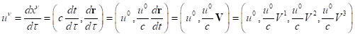
In (49), the following definitions of four-position and four-velocity with covariant indices, valid in the special theory of relativity, were
used:
![]() ,
, ![]() . (50)
. (50)
Similar expressions with a contravariant index have the following form:
![]() ,
,
 .
.
(51)
In (51), the velocity ![]() of motion of the center of momentum is expressed in terms of contravariant components in the form
of motion of the center of momentum is expressed in terms of contravariant components in the form ![]() . Note that expressions (51) are
considered primary in the sense that they are valid even in curved spacetime.
. Note that expressions (51) are
considered primary in the sense that they are valid even in curved spacetime.
Let us transform the four-velocity (51) of the system’s center of momentum into an expression with a covariant index using the metric tensor at
the center of
momentum:
![]() . (52)
. (52)
The four-velocity components (52) are as follows:
![]() .
.
![]() .
.
![]() .
.
![]() .
.
(53)
From (52-53) it is clear that even in the case when ![]() and the center of momentum is stationary in the reference frame
and the center of momentum is stationary in the reference frame ![]() , the spatial components
, the spatial components ![]() ,
, ![]() and
and ![]() , of four-velocity
, of four-velocity ![]() may not be equal to zero. A comparison of the
components of four-velocity
may not be equal to zero. A comparison of the
components of four-velocity ![]() (52-53) with the components of
(52-53) with the components of ![]() (51) shows that the spatial components of
(51) shows that the spatial components of ![]() in the general case change
asymmetrically with respect to the spatial components of
in the general case change
asymmetrically with respect to the spatial components of ![]() . This means that the relativistic
momentum
. This means that the relativistic
momentum ![]() of the system in (45) may not be directed along the velocity
of the system in (45) may not be directed along the velocity ![]() , and then the equality on the right
side of (49) does not hold.
, and then the equality on the right
side of (49) does not hold.
From the above it follows that the
four-momentum ![]() is represented by the sum of two
integral vectors, the generalized four-vector
is represented by the sum of two
integral vectors, the generalized four-vector ![]() (38) with components in (39-40), and four-vector
(38) with components in (39-40), and four-vector ![]() (46) with components in (47-48).
(46) with components in (47-48).
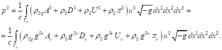
3.5. Components of four-momentum with contravariant index
The generalized four-momentum with a contravariant index can be
represented in terms of components as follows: ![]() . Then, the expressions for
. Then, the expressions for ![]() and
and ![]() follow from (41):
follow from (41):
 (54)
(54)
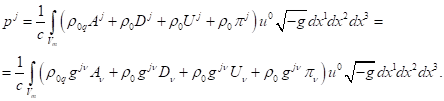 (55)
(55)
In (55), the index ![]() defines spaсe components of the generalized four-momentum with a contravariant
index. We can substitute into (54) the time components of fields’
four-potentials
defines spaсe components of the generalized four-momentum with a contravariant
index. We can substitute into (54) the time components of fields’
four-potentials ![]() ,
, ![]() ,
, ![]() and
and ![]() . In addition, only in Minkowski
spacetime, where metric tensor
. In addition, only in Minkowski
spacetime, where metric tensor ![]() has constant diagonal components
has constant diagonal components ![]() and other components are equal to zero, does
the time component
and other components are equal to zero, does
the time component ![]() (54) become equal to the time component
(54) become equal to the time component ![]() (39). In this case, the time component
(39). In this case, the time component ![]() up to a factor in the form of the speed of
light can be part of the energy
up to a factor in the form of the speed of
light can be part of the energy ![]() (36), defining the particles’ energy in scalar
field potentials. In this regard and in order to simplify the results, all the
subsequent arguments apply only to Minkowski spacetime.
(36), defining the particles’ energy in scalar
field potentials. In this regard and in order to simplify the results, all the
subsequent arguments apply only to Minkowski spacetime.
Let us determine a four-vector with a contravariant index ![]() . By analogy with (46), it should be
. By analogy with (46), it should be
![]() ,
, ![]() ,
, ![]() , (56)
, (56)
where the index ![]() .
.
The quantity ![]() (56) coincides with
(56) coincides with ![]() (47) because we are now writing the formulas
in Minkowski spacetime.
(47) because we are now writing the formulas
in Minkowski spacetime.
Like in (1), the system’s four-momentum with a contravariant index is
written as follows:
![]() . (57)
. (57)
In Minkowski
spacetime, the center of momentum of a physical system moves at a certain
constant velocity ![]() , which is part of four-velocity
(51). As in (49), we will again assume that the components of system’s momentum
, which is part of four-velocity
(51). As in (49), we will again assume that the components of system’s momentum
![]() (57) are directed along the components of
velocity
(57) are directed along the components of
velocity ![]() of motion of the system’s center of momentum, and the four-momentum
of motion of the system’s center of momentum, and the four-momentum ![]() is directed along the four-velocity
is directed along the four-velocity ![]() of motion of the system’s center of momentum:
of motion of the system’s center of momentum:
![]() .
(58)
.
(58)
In (58) ![]() denotes the system’s energy,
calculated using (36) in the center-of-momentum frame
denotes the system’s energy,
calculated using (36) in the center-of-momentum frame ![]() ;
; ![]() is the time component of
four-velocity of the center of momentum, taken with a contravariant index.
is the time component of
four-velocity of the center of momentum, taken with a contravariant index.
From (49) and (58), we can see that
different expressions for the same energy ![]() in the form
in the form ![]() and
and ![]() are possible because, only in the
special theory of relativity for time components of four-velocity with
covariant and contravariant indices, the following relation holds:
are possible because, only in the
special theory of relativity for time components of four-velocity with
covariant and contravariant indices, the following relation holds: ![]() , where
, where ![]() is the Lorentz factor of the
center of momentum. Moreover, four-momenta (49) and (58) are related by the
formula
is the Lorentz factor of the
center of momentum. Moreover, four-momenta (49) and (58) are related by the
formula ![]() , where
, where ![]() is the metric tensor of Minkowski
spacetime.
is the metric tensor of Minkowski
spacetime.
For a moving material point, the
standard expression for four-momentum is ![]() , where the metric tensor
, where the metric tensor ![]() is taken at the location of the
material point. Obviously, for a system with many particles, such a local
expression of the four-momentum
is taken at the location of the
material point. Obviously, for a system with many particles, such a local
expression of the four-momentum ![]() through the metric tensor
through the metric tensor ![]() at any one point turns out to be
unacceptable. For a system of particles, the expression
at any one point turns out to be
unacceptable. For a system of particles, the expression ![]() in (56), valid in the special theory
of relativity, should be used instead of
in (56), valid in the special theory
of relativity, should be used instead of ![]() . In curved spacetime, defining the four-momentum
. In curved spacetime, defining the four-momentum ![]() with the contravariant index
requires additional assumptions.
with the contravariant index
requires additional assumptions.
3.6. Relativistic uniform system at rest
Let us apply the formulas obtained
above to calculate the four-momentum of a physical system, which is a
relativistic uniform system. To simplify, we perform calculations in Minkowski
spacetime, that is, within the framework of the special theory of relativity.
The relativistic uniform system was
investigated in a number of papers [11], [21-22] and it has been well studied.
It is a physical system of spherical shape consisting of charged particles and
fields that is held in equilibrium by its own gravitational field and is
counteracted by electromagnetic field, acceleration field and pressure field.
All the mentioned fields are considered vector fields, and gravitation is
represented in the framework of covariant theory of gravitation [8], [23-25].
It is assumed that the particles are moving randomly and that the global vector
potentials ![]() ,
, ![]() ,
, ![]() , and
, and ![]() of all the fields in the
center-of-momentum frame
of all the fields in the
center-of-momentum frame ![]() are equal to zero. As a result,
in the sphere at rest, all solenoidal vectors, such as magnetic field and
torsion field (which is called gravitomagnetic field in theory of
gravitoelectromagnetism), are also equal to zero.
are equal to zero. As a result,
in the sphere at rest, all solenoidal vectors, such as magnetic field and
torsion field (which is called gravitomagnetic field in theory of
gravitoelectromagnetism), are also equal to zero.
Since the vector potentials in ![]() are equal to zero, then, according
to (40),
are equal to zero, then, according
to (40), ![]() . For the time component of generalized four-momentum (39), then in
. For the time component of generalized four-momentum (39), then in ![]() it was calculated in [17] in the
following form:
it was calculated in [17] in the
following form:
 , (59)
where ![]() is the Lorentz factor of particles at the
center of the sphere,
is the Lorentz factor of particles at the
center of the sphere, ![]() is acceleration field coefficient,
is acceleration field coefficient, ![]() is pressure field coefficient,
is pressure field coefficient, ![]() is radius of the sphere densely filled with
particles, and
is radius of the sphere densely filled with
particles, and ![]() is scalar potential of pressure field at the
center of the sphere. The mass
is scalar potential of pressure field at the
center of the sphere. The mass ![]() is sum of invariant masses of all the system’s
particles. This mass is equal to gravitational mass
is sum of invariant masses of all the system’s
particles. This mass is equal to gravitational mass ![]() of the system and is found with the help of
Lorentz factor
of the system and is found with the help of
Lorentz factor ![]() of particles, depending on the current radius.
The mass
of particles, depending on the current radius.
The mass ![]() is determined by the following formula:
is determined by the following formula:
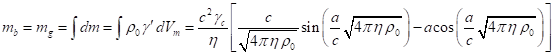 .
.
(60)
The total charge of the sphere is
calculated in a similar way as the sum of the invariant charges of all the particles, which are found in the particles’
comoving reference frames:
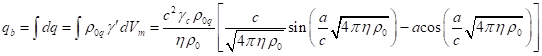 .
.
(61)
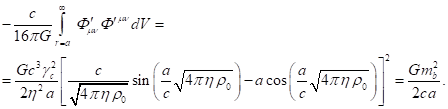
To calculate in
the center-of-momentum frame ![]() the fields’ energy
the fields’ energy ![]() , we use the results from [24], [26].
For volume, occupied by matter, we obtain the following:
, we use the results from [24], [26].
For volume, occupied by matter, we obtain the following:
(62)
According to [15], [21], in the system under consideration, the relation
between the field coefficients follows from the equation of particle motion:
![]() , (63)
, (63)
where ![]() is the electric constant.
is the electric constant.
If we sum the integrals of all
tensor invariants in (62) and take into account (63), we obtain zero:
 .
.
(64)
The equation (64) corresponds to the
fact that the energy ![]() in (30) becomes equal to zero.
Therefore, in the system under consideration, fields inside the matter will not
contribute to the component
in (30) becomes equal to zero.
Therefore, in the system under consideration, fields inside the matter will not
contribute to the component ![]() according to (47).
according to (47).
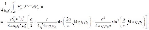
Outside matter there are only electromagnetic and gravitational fields,
for which instead of (62) taking into account (60-61) we can write:
(65)
(66)
The sum of (64), (65) and (66) gives the integral of the sum of tensor
invariants in (47), taking into account the fields inside and outside the
matter:
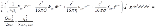
(67)
Taking into account (67) from (47) we find:
(68)
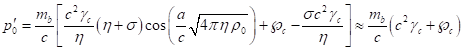
All the primed quantities are
calculated in the center-of-momentum frame ![]() associated with the center of the
sphere.
associated with the center of the
sphere.
Within the framework of the special
theory of relativity, the global scalar and vector field potentials inside a
sphere with chaotically moving particles obey the equations [16]:
![]() ,
, ![]() ,
,
![]() ,
, ![]() ,
,
![]() ,
, ![]() ,
,
![]() ,
, ![]() . (69)
. (69)
In a stationary and non-rotating
sphere under equilibrium conditions, the charge current density ![]() and mass current density
and mass current density ![]() are equal to zero, since it is
assumed that all physical quantities are independent of time, and the directed
flows of charge and mass necessary for the emergence of
are equal to zero, since it is
assumed that all physical quantities are independent of time, and the directed
flows of charge and mass necessary for the emergence of ![]() and
and ![]() are absent. As a consequence, the
vector potentials
are absent. As a consequence, the
vector potentials ![]() ,
, ![]() ,
, ![]() and
and ![]() of fields in (69) are equal to
zero. The scalar potentials
of fields in (69) are equal to
zero. The scalar potentials ![]() ,
, ![]() ,
, ![]() and
and ![]() of fields in (69) depend on the
square
of fields in (69) depend on the
square ![]() of the velocity of typical
particles at the observation point, since
of the velocity of typical
particles at the observation point, since ![]() is included in the Lorentz factor
is included in the Lorentz factor
![]() .
.
As a result, at ![]() in the limit of continuous medium, the global scalar field
potentials inside the sphere with randomly moving particles depend on the
velocity
in the limit of continuous medium, the global scalar field
potentials inside the sphere with randomly moving particles depend on the
velocity ![]() of typical particles up to terms
containing the square
of typical particles up to terms
containing the square ![]() of the speed of light in the
denominator.
of the speed of light in the
denominator.
According to (28), the Lagrangian density
![]() depends on the field tensors, each of which is found by calculating the
four-rotor from the corresponding four-potential containing scalar and vector
potentials. Therefore, in the reference frame
depends on the field tensors, each of which is found by calculating the
four-rotor from the corresponding four-potential containing scalar and vector
potentials. Therefore, in the reference frame ![]() , part
, part ![]() of the Lagrangian density and the
corresponding part of the Lagrangian function
of the Lagrangian density and the
corresponding part of the Lagrangian function ![]() have some weak dependence on velocity
have some weak dependence on velocity ![]() . In (68) it is required to find the derivatives
. In (68) it is required to find the derivatives ![]() with respect to the velocities of
particles from the field potentials, and when calculating the sum
with respect to the velocities of
particles from the field potentials, and when calculating the sum 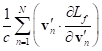 it is necessary to find the
derivatives
it is necessary to find the
derivatives ![]() with respect to the
velocities
with respect to the
velocities ![]() of typical particles.
of typical particles.
This leads to the fact that the time
component ![]() (68) acquires small additional
terms containing the square of the speed of light in the denominator. In order
to simplify calculations, we will not consider such terms, leaving only the
main terms.
(68) acquires small additional
terms containing the square of the speed of light in the denominator. In order
to simplify calculations, we will not consider such terms, leaving only the
main terms.
As a result, the time component ![]() (68) in
(68) in ![]() will be approximately equal to
will be approximately equal to
![]() . (70)
. (70)
In ![]() relation (46)
must hold for energies:
relation (46)
must hold for energies: ![]() . Hence, taking into account (59)
and (70), the energy of the sphere at rest will be equal to:
. Hence, taking into account (59)
and (70), the energy of the sphere at rest will be equal to:
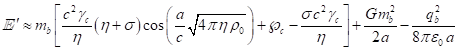 . (71)
According to (71), the relativistic
energy ![]() of the system at rest is
expressed in terms of the total energy of particles in field potentials minus
the energy of gravitational and electromagnetic fields outside the matter.
of the system at rest is
expressed in terms of the total energy of particles in field potentials minus
the energy of gravitational and electromagnetic fields outside the matter.
Since in ![]() both the total momentum, and the
generalized momentum are equal to zero,
both the total momentum, and the
generalized momentum are equal to zero, ![]() , and
, and ![]() , then according to (46) the field momentum will be equal to zero:
, then according to (46) the field momentum will be equal to zero: ![]() .
.
For a fixed sphere ![]() , the Lorentz factor
, the Lorentz factor ![]() , the time component of four-velocity of sphere
, the time component of four-velocity of sphere ![]() , and four-momentum (49) in
, and four-momentum (49) in ![]() are written as follows:
are written as follows:
![]() .
(72)
.
(72)
3.7. Moving relativistic uniform system
In [17], transformation of the
four-velocity of an arbitrary particle from ![]() to inertial reference frame
to inertial reference frame ![]() was carried out using Lorentz
transformations for the case, when the sphere with particles was moving at
constant velocity
was carried out using Lorentz
transformations for the case, when the sphere with particles was moving at
constant velocity ![]() along the axis
along the axis ![]() :
:
![]() (73)
(73)
![]() ,
,
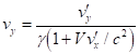 ,
,
![]() ,
,
![]() .
.
(74)
Here, ![]() denotes the Lorentz factor of the
particle in
denotes the Lorentz factor of the
particle in ![]() ;
; ![]() ,
, ![]() and
and ![]() are the components of the particle’s velocity in
are the components of the particle’s velocity in ![]() ;
; ![]() is the Lorentz factor of the center
of momentum, which moves together with the physical system at velocity
is the Lorentz factor of the center
of momentum, which moves together with the physical system at velocity ![]() ;
; ![]() is the Lorentz factor of a particle in the center-of-the
momentum frame
is the Lorentz factor of a particle in the center-of-the
momentum frame ![]() ;
; ![]() ,
, ![]() and
and ![]() are the components of the
particle’s velocity in
are the components of the
particle’s velocity in ![]() .
.
In (73), the time component of the
four-velocity of particle is ![]() . Using this in (38-40), after transformation of fields’ four-potentials
from the reference frame
. Using this in (38-40), after transformation of fields’ four-potentials
from the reference frame ![]() into
into ![]() and then averaging over the
velocities
and then averaging over the
velocities ![]() of randomly and multidirectional
moving particles, the following was found in [17]:
of randomly and multidirectional
moving particles, the following was found in [17]:
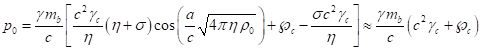 . (75)
In comparison with (59), the
component ![]() (75) is increased by a factor
of
(75) is increased by a factor
of ![]() due to the motion of the physical system as a
whole at velocity
due to the motion of the physical system as a
whole at velocity ![]() . Moreover, the relation
. Moreover, the relation ![]() is satisfied. Thus, in
is satisfied. Thus, in ![]() we find all the components of the generalized four-momentum
for a sphere with particles moving at constant velocity
we find all the components of the generalized four-momentum
for a sphere with particles moving at constant velocity ![]() along the axis
along the axis ![]() :
: ![]() .
.
Now we need to calculate the
components of the four-vector![]() , associated with the energy and
momentum of the fields, both in the matter and beyond. According to (47), the
time component
, associated with the energy and
momentum of the fields, both in the matter and beyond. According to (47), the
time component ![]() is found using field
four-potentials and field tensors; moreover, to calculate the field tensors the
strengths and solenoidal vectors in
is found using field
four-potentials and field tensors; moreover, to calculate the field tensors the
strengths and solenoidal vectors in ![]() are needed.
are needed.
There are two
equivalent methods for determining strengths and solenoidal vectors in ![]() . In the first of them, we can take
these quantities in
. In the first of them, we can take
these quantities in ![]() and then apply the transformation of tensor
components from
and then apply the transformation of tensor
components from ![]() into
into ![]() . The other method involves first
transforming the fields’ four-potentials from
. The other method involves first
transforming the fields’ four-potentials from ![]() to
to ![]() using Lorentz
transformations, and then calculating the strengths and solenoidal vectors in
using Lorentz
transformations, and then calculating the strengths and solenoidal vectors in ![]() using these four-potentials with the help of
four-curl.
using these four-potentials with the help of
four-curl.
For clarity, we use the first method and find the components of
electromagnetic tensor in ![]() .
.
In Cartesian coordinates, even in curved
spacetime, the following relations are valid for the components of electric
field strength ![]() , magnetic field induction
, magnetic field induction ![]() and electromagnetic field tensor
and electromagnetic field tensor ![]() with covariant indices:
with covariant indices:
![]() ,
, ![]() .
(76)
.
(76)
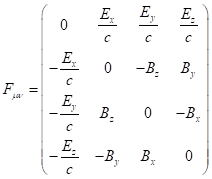 . (77)
The electromagnetic field tensor
with contravariant indices can be found, knowing the components of ![]() in (77) and the metric tensor
in (77) and the metric tensor ![]() , using the formula:
, using the formula:
![]() .
(78)
.
(78)
In the special theory of relativity,
the metric tensor ![]() becomes equal to the tensor
becomes equal to the tensor ![]() of the following form:
of the following form:
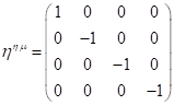 . (79)
Substitution of (77) and (79) into
(78) gives the tensor expression:
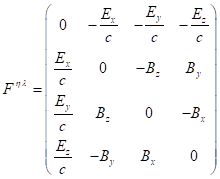 . (80)
Let us consider relations (76) in the reference frame ![]() .Since the global vector potentials
.Since the global vector potentials ![]() ,
, ![]() ,
, ![]() and
and ![]() of fields in
of fields in ![]() are equal to
zero, as follows from (69), the vector of electric field strength
are equal to
zero, as follows from (69), the vector of electric field strength ![]() inside the
sphere at rest is expressed in (76)in terms of the
scalar electric potential
inside the
sphere at rest is expressed in (76)in terms of the
scalar electric potential ![]() , found in [26], according to
standard formula for electrostatics:
, found in [26], according to
standard formula for electrostatics:
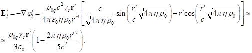
(81)
In (81) ![]() is the current radius inside the
sphere, and the index
is the current radius inside the
sphere, and the index ![]() indicates that the strength
indicates that the strength ![]() and scalar potential
and scalar potential ![]() refer to the internal field of
the sphere. Since
refer to the internal field of
the sphere. Since ![]() , then according to (76) in
, then according to (76) in ![]() the magnetic field is equal to zero everywhere,
the magnetic field is equal to zero everywhere, ![]() .
.
The components of the antisymmetric
electromagnetic tensor ![]() in
in ![]() in the special theory of relativity are expressed
according to (80) in terms of components of vectors
in the special theory of relativity are expressed
according to (80) in terms of components of vectors ![]() and
and ![]() as follows:
as follows:
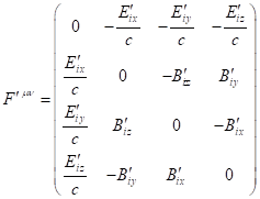 . (82)
![]() ,
, ![]() ,
,
![]() ,
,
![]() ,
, ![]() ,
, ![]() .
.
(83)
The Lorentz transformation of tensor
components from ![]() to
to ![]() is carried out according to
standard formulas (§ 24. Lorentz transformation of the field, in [2]):
is carried out according to
standard formulas (§ 24. Lorentz transformation of the field, in [2]):
![]() ,
, ![]() ,
,
![]() ,
,
![]() ,
, ![]() ,
,
![]() . (84)
. (84)
Substituting
(83) into (84), in view of relations ![]() ,
, ![]() , and
, and ![]() , gives the following:
, gives the following:
![]() ,
, ![]() ,
, ![]() ,
,
![]() ,
, ![]() ,
, ![]() . (85)
. (85)
According to (85), due to the motion of the sphere with an internal
electric field, a magnetic field appears in the reference frame ![]() , although in the reference frame
, although in the reference frame ![]() associated with the sphere there is no
magnetic field. This is a consequence of the principle of relativity in
relation to the components of the electromagnetic field, when the own electric
field of a moving object generates an additional magnetic field in another
reference frame, and the own magnetic field of a moving object generates an
additional electric field in another reference frame. In this case, the
additional fields turn out to be proportional to the velocity
associated with the sphere there is no
magnetic field. This is a consequence of the principle of relativity in
relation to the components of the electromagnetic field, when the own electric
field of a moving object generates an additional magnetic field in another
reference frame, and the own magnetic field of a moving object generates an
additional electric field in another reference frame. In this case, the
additional fields turn out to be proportional to the velocity ![]() of the object.
of the object.
The contribution to ![]() (47) from the tensor invariant of
electromagnetic field in the reference frame
(47) from the tensor invariant of
electromagnetic field in the reference frame ![]() is as follows:
is as follows:
![]() . (86)
. (86)
In (86), expressions ![]() (77) and
(77) and ![]() (80) were taken into account, for which we
obtain
(80) were taken into account, for which we
obtain![]() .
.
The subscript ![]() in
in ![]() and in
and in ![]() (86) indicates that the electric field
strength and magnetic field induction are taken inside the moving sphere. The
magnetic constant
(86) indicates that the electric field
strength and magnetic field induction are taken inside the moving sphere. The
magnetic constant ![]() and the electric constant
and the electric constant ![]() are related to each other and to the square of the speed of light by
the relation
are related to each other and to the square of the speed of light by
the relation ![]() .
.
Let us calculate the quantities ![]() and
and ![]() using the components
using the components ![]() and
and ![]() (85), and substitute
(85), and substitute ![]() and
and ![]() in (86), taking into account the expression
for the Lorentz factor
in (86), taking into account the expression
for the Lorentz factor ![]() :
:
![]() . (87)
. (87)
In contrast to
(62), in (87) the integration is carried out over the moving volume of the
sphere. A moving sphere in the special theory of relativity is considered a
Heaviside ellipsoid. Like in [27-28], we introduce in ![]() new coordinates
new coordinates ![]() , associated with Cartesian
coordinates:
, associated with Cartesian
coordinates:
![]() ,
, ![]() ,
, ![]() . (88)
. (88)
The volume element in these coordinates is defined by the formula ![]() . The equation of the Heaviside
ellipsoid surface, in view of (88), is as follows:
. The equation of the Heaviside
ellipsoid surface, in view of (88), is as follows:
![]() ,
, ![]() . (89)
. (89)
Thus, the
limits of integration over the sphere’s volume in new coordinates will be as
follows: radius ![]() should vary
from 0 to
should vary
from 0 to ![]() , and angles
, and angles ![]() and
and ![]() vary the same as in spherical coordinates
(from 0 to
vary the same as in spherical coordinates
(from 0 to ![]() for the angle
for the angle ![]() and from 0 to
and from 0 to ![]() for the angle
for the angle ![]() ).
).
If in ![]() we denote the current radius by
we denote the current radius by ![]() , and express the coordinates
, and express the coordinates ![]() in terms of the coordinates
in terms of the coordinates ![]() in
in ![]() with the help of Lorentz transformations and
use (88), we obtain the following:
with the help of Lorentz transformations and
use (88), we obtain the following:
![]() . (90)
. (90)
According to
(90), instead of ![]() we can use the
coordinate
we can use the
coordinate ![]() in (81), after which we can substitute the
vector
in (81), after which we can substitute the
vector ![]() into (87). Considering the relation
into (87). Considering the relation ![]() , we obtain:
, we obtain:
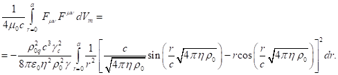 (91)
(91)
Similarly, we can repeat the same steps for remaining fields. In ![]() gravitational
field strength inside the sphere, strengths of acceleration field and pressure
field are expressed in terms of scalar potentials, as found in [24], [26],
[29]:
gravitational
field strength inside the sphere, strengths of acceleration field and pressure
field are expressed in terms of scalar potentials, as found in [24], [26],
[29]:
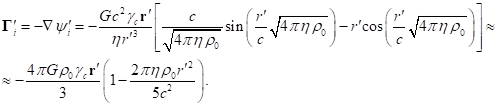
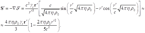
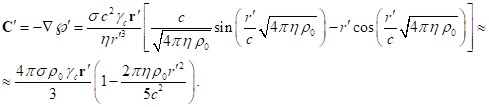
(92)
Like in (84-85), the field’s strengths and solenoidal vectors in the
reference frame ![]() are equal to:
are equal to:
![]() ,
, ![]() ,
, ![]() ,
,
![]() ,
, ![]() ,
, ![]() .
.
![]() ,
, ![]() ,
, ![]() ,
,
![]() ,
, ![]() ,
, ![]() .
.
![]() ,
, ![]() ,
, ![]() ,
,
![]() ,
, ![]() ,
, ![]() .
.
(93)
Taking into account (86-91), as well
as (92-93), the results of integrating tensor invariants over the moving
sphere’s volume for three remaining fields are as follows:
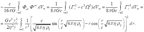
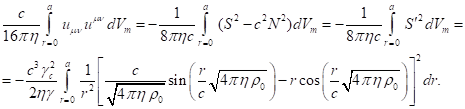
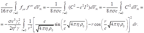
(94)
Let us sum the terms in (91) and (94) and take into account (63):
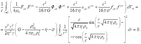
(95)
Sum (95) is
included as an integral part in ![]() (47). Thus, in matter inside the moving sphere the sum of contributions to
(47). Thus, in matter inside the moving sphere the sum of contributions to ![]() from all the fields becomes equal to zero, as
in the case of the sphere at rest when summing integrals of all tensor
invariants in (64).
from all the fields becomes equal to zero, as
in the case of the sphere at rest when summing integrals of all tensor
invariants in (64).
Now it is necessary to consider in ![]() electromagnetic
and gravitational fields outside the sphere. In the center-of-momentum frame
electromagnetic
and gravitational fields outside the sphere. In the center-of-momentum frame ![]() , there are both an external electric
field strength and an external gravitational field strength:
, there are both an external electric
field strength and an external gravitational field strength:
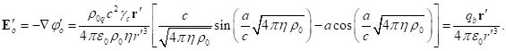
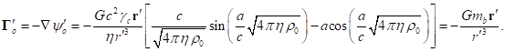
(96)
In (96), the index ![]() indicates that a quantity refers
to space outside the matter. In the reference frame
indicates that a quantity refers
to space outside the matter. In the reference frame ![]() , in which the sphere is moving at
constant velocity
, in which the sphere is moving at
constant velocity ![]() along the axis
along the axis ![]() , similar to (85) and (93) a magnetic field
, similar to (85) and (93) a magnetic field ![]() appears, as does a torsion field
appears, as does a torsion field ![]() :
:
![]() ,
, ![]() ,
, ![]() ,
,
![]() ,
, ![]() ,
, ![]() .
.
![]() ,
, ![]() ,
, ![]() ,
,
![]() ,
, ![]() ,
, ![]() . (97)
. (97)
Taking into account relations
(87-90), as well as (97) and the relation ![]() , for integrals of tensor invariants of external fields of moving sphere
we find the following:
, for integrals of tensor invariants of external fields of moving sphere
we find the following:
![]()

(98)
Substituting (98) into (47) and
taking into account (95) for the fields inside the sphere, in ![]() we determine the time component
we determine the time component ![]() :
:
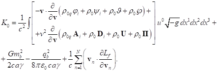 (99)
(99)
In the system under consideration ![]() ,
, ![]() , and the continuous medium approximation is used, while in the
center-of-momentum frame
, and the continuous medium approximation is used, while in the
center-of-momentum frame ![]() , in accordance with (69), the vector potentials are considered equal to
zero. At the same time, the scalar field potentials at the location of a
particle weakly depend on the speed
, in accordance with (69), the vector potentials are considered equal to
zero. At the same time, the scalar field potentials at the location of a
particle weakly depend on the speed ![]() of this particle, and are
determined up to terms containing the square of the speed of light in the
denominator. The situation does not
change in the reference frame
of this particle, and are
determined up to terms containing the square of the speed of light in the
denominator. The situation does not
change in the reference frame ![]() ; although potentials become dependent on the velocity
; although potentials become dependent on the velocity ![]() of the sphere’s motion, they
still weakly depend on the components of particles’ velocity
of the sphere’s motion, they
still weakly depend on the components of particles’ velocity ![]() presented in (74). Neglecting
small terms, we find an approximate expression for
presented in (74). Neglecting
small terms, we find an approximate expression for ![]() (99):
(99):
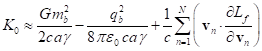 . (100)
Let us
represent ![]() in the form
in the form ![]() . Inside the sphere, taking into account (2) and (28), as well as
conditions for energy gauging and metrics [11], [20] in the form
. Inside the sphere, taking into account (2) and (28), as well as
conditions for energy gauging and metrics [11], [20] in the form ![]() , we obtain:
, we obtain:
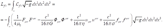
(101)
If we take into account (95), then inside the moving sphere we obtain ![]() , so that in this case
, so that in this case ![]() (101) does not contribute to
(101) does not contribute to ![]() in (100). In view of (98), we
find
in (100). In view of (98), we
find ![]() in space outside the sphere,
where there are only electromagnetic and gravitational fields:
in space outside the sphere,
where there are only electromagnetic and gravitational fields:
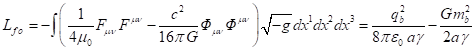 . (102)
In (102) the Lorentz factor ![]() is present, which is a function
of the velocity
is present, which is a function
of the velocity ![]() of the sphere motion along the
axis
of the sphere motion along the
axis ![]() of reference frame
of reference frame ![]() .
.
According to (74), the particle velocity in ![]() is equal to:
is equal to:
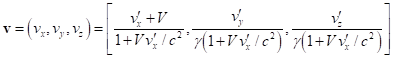 . (103)
If we average velocities ![]() of neighboring particles directed in all
directions, in (103) we obtain
of neighboring particles directed in all
directions, in (103) we obtain ![]() . This can be explained by the
following calculations:
. This can be explained by the
following calculations:
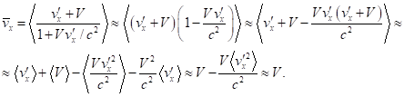 (104)
(104)
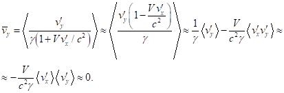
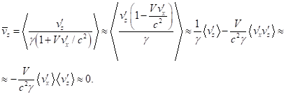
(105)
In (104) it is assumed that after averaging over all directions ![]() , and that the small term
, and that the small term ![]() can be neglected. In (105), it is similarly
assumed that the average values of
can be neglected. In (105), it is similarly
assumed that the average values of ![]() and
and ![]() , , and can be neglected by small terms containing the square of the speed
of light in the denominator.
, , and can be neglected by small terms containing the square of the speed
of light in the denominator.
Since ![]() ,
, ![]() , in (100) it is necessary to calculate the sum
, in (100) it is necessary to calculate the sum 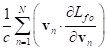 , including the derivative
 ![]() with respect to the particles’
velocities
with respect to the particles’
velocities ![]() .
.
However, ![]() is a result of averaging over the
velocities of individual particles, and to a first approximation depends only
on
is a result of averaging over the
velocities of individual particles, and to a first approximation depends only
on ![]() . Fields outside the sphere look as if they are created by one body
without internal motion of particles, and this body moves at velocity
. Fields outside the sphere look as if they are created by one body
without internal motion of particles, and this body moves at velocity ![]() and has a mass and charge equal
to the sum of the masses and charges of individual particles of the system.
This allows us to replace this sum with its average value by replacing
and has a mass and charge equal
to the sum of the masses and charges of individual particles of the system.
This allows us to replace this sum with its average value by replacing ![]() with
with ![]() :
:
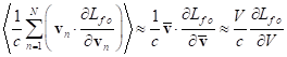
To better understand (106), we can consider the electromagnetic field
outside a moving sphere with radius ![]() , uniformly and symmetrically filled
with a large number
, uniformly and symmetrically filled
with a large number ![]() of charged particles, each of which has a
charge
of charged particles, each of which has a
charge ![]() . Due to symmetry taking into
account Gauss's theorem, the field outside the sphere will be the same as if
all the charges of the sphere were placed at the center of the sphere and there
would be the charge
. Due to symmetry taking into
account Gauss's theorem, the field outside the sphere will be the same as if
all the charges of the sphere were placed at the center of the sphere and there
would be the charge ![]() . So the
sphere with
. So the
sphere with ![]() charges in relation to the field outside the
sphere becomes equivalent to one charge
charges in relation to the field outside the
sphere becomes equivalent to one charge ![]() , which has a point particle radius
much smaller than the radius
, which has a point particle radius
much smaller than the radius ![]() . In this case, we can assume that
the sum in (106) contains only one term for one particle with charge
. In this case, we can assume that
the sum in (106) contains only one term for one particle with charge ![]() , and
, and ![]() is a Lagrange function for a
point charged particle moving with the velocity
is a Lagrange function for a
point charged particle moving with the velocity ![]() . The field of such a particle with
the charge
. The field of such a particle with
the charge ![]() is equivalent to the field of the moving
sphere, which allows us to replace the sum of terms in (106) by one term.
is equivalent to the field of the moving
sphere, which allows us to replace the sum of terms in (106) by one term.
Substituting into (106) ![]() from (102), taking into account the expression for the Lorentz
factor
from (102), taking into account the expression for the Lorentz
factor ![]() , we find:
, we find:
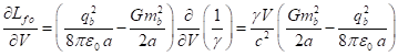 .
.
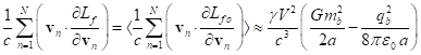 . (107)
This sum (107) is presented in (100), which allows us to clarify the
form ![]() :
:
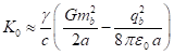 .
(108)
.
(108)

(109)
By comparing
(109) and (71) for the case of the sphere at rest we can see that the energy of moving sphere increases by a factor of ![]() .
.
Now we use (48) to calculate the vector ![]() , again assuming that the charge density, mass density, and field
potentials inside the moving sphere in the first approximation do not depend on
velocities of individual particles at the integration point. Then in (48) the
integral vanishes and the following equation holds:
, again assuming that the charge density, mass density, and field
potentials inside the moving sphere in the first approximation do not depend on
velocities of individual particles at the integration point. Then in (48) the
integral vanishes and the following equation holds:
 .
(110)
.
(110)
In (110) ![]() , and from (95) it follows that inside the sphere
, and from (95) it follows that inside the sphere ![]() in (101) is equal to zero.
Considering the average value of the sum in (110), taking into account the
expression for velocity
in (101) is equal to zero.
Considering the average value of the sum in (110), taking into account the
expression for velocity ![]() , the value
, the value ![]() (102) and
(102) and ![]() , we find:
, we find:
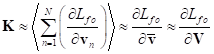 ,
,
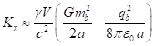 ,
, ![]() ,
, ![]() . (111)
. (111)
Comparison of (108) and (111) gives the
relations:
![]() ,
, ![]() . (112)
. (112)
In (75), the
component ![]() was calculated, which allows determination of
the component
was calculated, which allows determination of
the component ![]() for generalized four-momentum
for generalized four-momentum ![]() of moving sphere:
of moving sphere:
![]() ,
, ![]() . (113)
. (113)
Relations (112)
for ![]() have the same form as relations for
have the same form as relations for ![]() in (113).
in (113).
Adding
vectors ![]() and
and ![]() according
to (46), we find the momentum of the system:
according
to (46), we find the momentum of the system:
 . (114)
According to the method of its calculation in (13), the generalized
four-momentum ![]() (113) is a nonlocal four-vector of integral
type with a covariant index associated with the interaction of particles with
each other and with fields. Nonlocality of
(113) is a nonlocal four-vector of integral
type with a covariant index associated with the interaction of particles with
each other and with fields. Nonlocality of ![]() is a consequence of its definition through the
integral over the volume occupied by all typical particles of the system. The
four-vector
is a consequence of its definition through the
integral over the volume occupied by all typical particles of the system. The
four-vector ![]() (112), which specifies the four-momentum of
the fields of the system, has the same properties. The sum of
four-vectors
(112), which specifies the four-momentum of
the fields of the system, has the same properties. The sum of
four-vectors ![]() and
and ![]() в (46) gives the total four-momentum of the physical system
в (46) gives the total four-momentum of the physical system ![]() with the covariant index.
with the covariant index.
3.8. Integral vector inside moving
sphere
In [7] we calculated the integral
vector ![]() (9) for a fixed sphere within the
framework of the special theory of relativity. Now we determine this vector for
the case of motion of the sphere with particles at constant velocity
(9) for a fixed sphere within the
framework of the special theory of relativity. Now we determine this vector for
the case of motion of the sphere with particles at constant velocity ![]() along the
along the ![]() axis in the reference frame
axis in the reference frame ![]() . The stress-energy tensor of a physical system consists of the sum of
the stress-energy tensors of electromagnetic and gravitational fields,
acceleration field and pressure field. Taking into account the metric signature
. The stress-energy tensor of a physical system consists of the sum of
the stress-energy tensors of electromagnetic and gravitational fields,
acceleration field and pressure field. Taking into account the metric signature
![]() we use, we can write:
we use, we can write:
![]() . (115)
. (115)
![]() ,
,
![]() ,
,
![]() ,
,
![]() . (116)
. (116)
The expression for the energy-momentum tensor ![]() of a physical system in (115)
follows from the principle of least action [11], and the tensor
of a physical system in (115)
follows from the principle of least action [11], and the tensor ![]() is included in the equation for
calculating the metric tensor
is included in the equation for
calculating the metric tensor ![]() . In (116)
. In (116) ![]() ,
, ![]() ,
, ![]() and
and ![]() are, respectively, the
energy-momentum tensors of the electromagnetic and gravitational fields, the
acceleration field and the pressure field. In this case, the tensor
are, respectively, the
energy-momentum tensors of the electromagnetic and gravitational fields, the
acceleration field and the pressure field. In this case, the tensor ![]() is expressed through the
electromagnetic field tensor
is expressed through the
electromagnetic field tensor ![]() , the tensor
, the tensor ![]() is expressed through the
gravitational field tensor
is expressed through the
gravitational field tensor ![]() , the tensor
, the tensor ![]() is expressed through the
acceleration field tensor
is expressed through the
acceleration field tensor ![]() , and the tensor
, and the tensor ![]() is expressed through the
pressure field tensor
is expressed through the
pressure field tensor ![]() . In (116)
. In (116) ![]() is the speed of light,
is the speed of light, ![]() is electrical constant,
is electrical constant, ![]() is gravitational constant,
is gravitational constant, ![]() and
and ![]() are constant of acceleration
field and pressure field, respectively.
are constant of acceleration
field and pressure field, respectively.
Let us first consider the situation
inside the sphere, that is, in its continuously distributed matter. We
calculate components ![]() ,
, ![]() ,
, ![]() and
and ![]() of fields’ stress-energy tensors
and consider that in Minkowski spacetime metric tensor
of fields’ stress-energy tensors
and consider that in Minkowski spacetime metric tensor ![]() becomes the metric tensor
becomes the metric tensor ![]() (79), which does not depend on time or coordinates.
(79), which does not depend on time or coordinates.
In Cartesian coordinates, the time components of the stress-energy
tensor of electromagnetic field in (116) can be written in terms of electric
field ![]() and magnetic field
and magnetic field ![]() :
:
![]() ,
, ![]() ,
,
![]() ,
, ![]() . (117)
. (117)
In (117), the vector ![]() is the cross product of the vectors
is the cross product of the vectors ![]() and
and ![]() ;
; ![]() denotes the projection of the vector
denotes the projection of the vector ![]() onto the
onto the ![]() axis of the Cartesian coordinate system.
Similarly,
axis of the Cartesian coordinate system.
Similarly, ![]() is a projection of the vector
is a projection of the vector ![]() onto the
onto the ![]() axis, and
axis, and ![]() is a projection of the vector
is a projection of the vector ![]() onto the
onto the ![]() axis of the Cartesian coordinate system.
axis of the Cartesian coordinate system.
If we take into account the definition of the Poynting vector in the
form ![]() and relation
and relation ![]() , then (117) can be represented in
standard form as follows:
, then (117) can be represented in
standard form as follows:
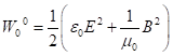 ,
, ![]() ,
, ![]() ,
, ![]() .
.
(118)
Substitution of components ![]() and
and ![]() (85) into (117) taking into account (81) and
the relation
(85) into (117) taking into account (81) and
the relation ![]() gives inside a moving sphere:
gives inside a moving sphere:
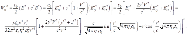
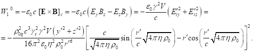

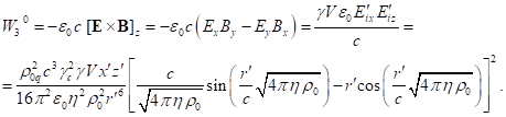 (119)
(119)
Similarly to (117), the time components of the stress-energy tensors of
gravitational field, acceleration field and pressure field in (116) can be
written in terms of strengths and solenoidal vectors of corresponding fields
[11]:
![]() ,
, ![]() ,
,
![]() ,
, ![]() .
.
![]() ,
, ![]() ,
,
![]() ,
, ![]() .
.
![]() ,
, ![]() ,
,
![]() ,
, ![]() . (120)
. (120)
In (120) ![]() and
and ![]() are the strength and torsion field of
gravitational field;
are the strength and torsion field of
gravitational field; ![]() and
and ![]() are the strength and solenoidal vector of
acceleration field;
are the strength and solenoidal vector of
acceleration field; ![]() and
and ![]() are the strength and solenoidal vector of
pressure field.
are the strength and solenoidal vector of
pressure field.
Let us
substitute (93) into (120) and take into account (92):
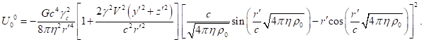
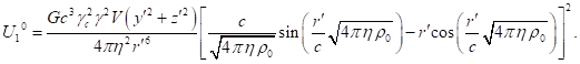
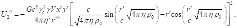
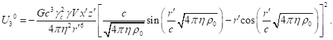
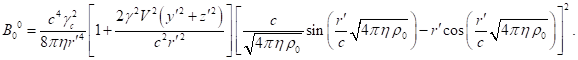
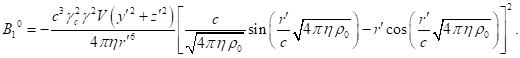
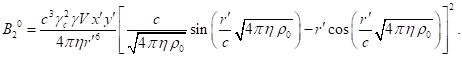
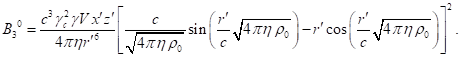
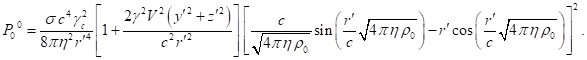
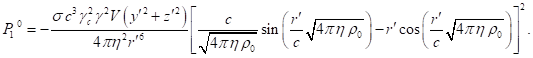
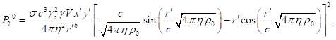
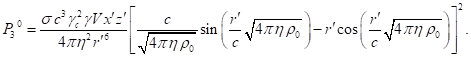 (121)
(121)
If we
substitute (119) and (121) into (115) and find the time components of the total
stress-energy tensor ![]() , then by integrating
, then by integrating ![]() over volume of moving sphere, according to (9), we can find the components
of the integral vector
over volume of moving sphere, according to (9), we can find the components
of the integral vector ![]() inside the sphere:
inside the sphere:
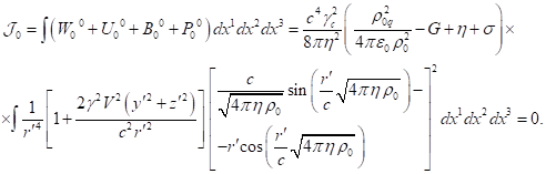
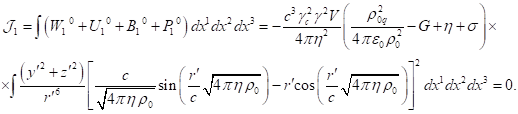
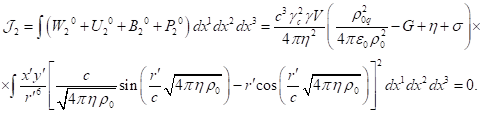
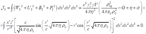
(122)
Before each integral in (122), in the corresponding bracket, there is a
sum which, according to (63), is equal to zero: ![]() .
.
This equality, containing field coefficients, was found in [15], [21],
as a consequence of the balance of forces from all fields acting on typical
particles.
Thus, inside moving sphere the
integral vector becomes equal to zero, ![]() .
.
3.9. Integral vector outside moving
sphere
To calculate the total integral
vector ![]() , it is necessary to integrate
, it is necessary to integrate ![]() over entire volume, both inside
and outside the sphere. Since acceleration field and pressure field are present
only in matter, only electromagnetic and gravitational fields remain outside
the sphere. Let us find the time components of the stress-energy tensors of
these fields, taking into account (117), (120), (96-97):
over entire volume, both inside
and outside the sphere. Since acceleration field and pressure field are present
only in matter, only electromagnetic and gravitational fields remain outside
the sphere. Let us find the time components of the stress-energy tensors of
these fields, taking into account (117), (120), (96-97):
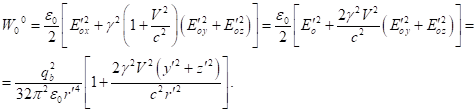
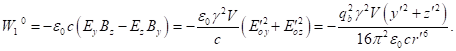
![]() .
.
![]() .
.
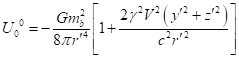 ,
, 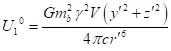 ,
,
![]() ,
, ![]() . (123)
. (123)
By substituting ![]() and
and ![]() from (123) into (115), we find
from (123) into (115), we find ![]() and the component
and the component ![]() in (9):
in (9):
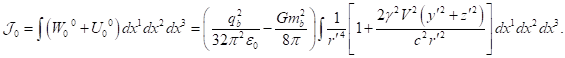
(124)
The integral in (124) is taken over
the volume outside the moving sphere, and the sphere is considered a Heaviside
ellipsoid. According to (90), we suppose that ![]() , where
, where ![]() is current radius in the reference
frame
is current radius in the reference
frame ![]() , associated with the center of
sphere, and
, associated with the center of
sphere, and ![]() is radial coordinate in (88). From
Lorentz transformations, in the case of the sphere’s motion at constant
velocity
is radial coordinate in (88). From
Lorentz transformations, in the case of the sphere’s motion at constant
velocity ![]() along the axis
along the axis ![]() in reference frame
in reference frame ![]() , it follows that
, it follows that ![]() ,
, ![]() , and
, and ![]() . Then, in view of (88), we have:
. Then, in view of (88), we have:
![]() ,
,
![]() ,
,
![]() ,
,
![]() . (125)
. (125)
As in (91), the volume element will
equal ![]() . Using all this in (124), we find:
. Using all this in (124), we find:
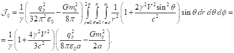 (126)
(126)
For space components of the integral vector ![]() in (9), using (123) and (125) we find the
following in a similar way:
in (9), using (123) and (125) we find the
following in a similar way:
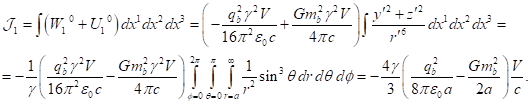
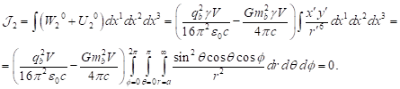
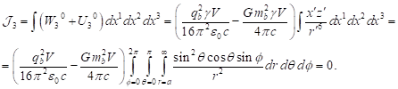 (127)
(127)
4. Discussion of results
In (122) we
found that in the matter inside a sphere all the components of the integral
vector ![]() become equal to zero. Therefore, it suffices
to consider only the components of the integral vector outside the matter.
become equal to zero. Therefore, it suffices
to consider only the components of the integral vector outside the matter.
According to (111-112) and (127), we have the following:
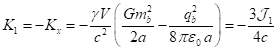 .
(128)
.
(128)
Comparison of
(108) and (126) gives:
![]() . (129)
. (129)
From (128) it
follows that the space component ![]() of the integral vector
of the integral vector ![]() is proportional to the space component
is proportional to the space component ![]() of the four-vector
of the four-vector ![]() , which defines contribution of
fields to energy-momentum of the system under consideration. According to (112), the relation
, which defines contribution of
fields to energy-momentum of the system under consideration. According to (112), the relation ![]() holds for components of four-vector
holds for components of four-vector ![]() .
.
However, for the components of the integral vector, according to
(126-127), we obtain a different relation:
![]() . (130)
. (130)
From (130) it
follows that the component ![]() depends in a complex manner on the velocity
depends in a complex manner on the velocity ![]() of the sphere’s motion. Even in the limit of low velocities in (130), we obtain a coefficient
of the sphere’s motion. Even in the limit of low velocities in (130), we obtain a coefficient ![]() that is not equal to unity, in contrast to the relation
that is not equal to unity, in contrast to the relation ![]() for components
of the four-vector
for components
of the four-vector ![]() , where similar coefficient is equal to 1. Thus, the integral vector
, where similar coefficient is equal to 1. Thus, the integral vector ![]() is not a four-vector; therefore, the integral
vector cannot specify either the four-momentum of the system or the four-momentum of the fields.
is not a four-vector; therefore, the integral
vector cannot specify either the four-momentum of the system or the four-momentum of the fields.
The same can be said in other words. According to (9), the integral
vector is obtained by volume integration of the time components ![]() of the total stress-energy tensor of the
system. Hence, it is not enough to know the stress-energy tensor of a system to
calculate the four-momentum.
of the total stress-energy tensor of the
system. Hence, it is not enough to know the stress-energy tensor of a system to
calculate the four-momentum.
On the other hand, the 4/3 factor in (130) is associated with the
so-called 4/3 problem, according to which the mass-energy contained in ![]() is approximately 4/3 times greater than the
mass-energy contained in component
is approximately 4/3 times greater than the
mass-energy contained in component ![]() . Obviously, such behavior of
mass-energies is inconsistent with the role of mass in the four-momentum of a
single point particle, where the mass is part of both energy and momentum to
the same extent.
. Obviously, such behavior of
mass-energies is inconsistent with the role of mass in the four-momentum of a
single point particle, where the mass is part of both energy and momentum to
the same extent.
In this case, what does the integral vector ![]() represent? According to its meaning, it is a volume integral of the equation of
motion, and it was shown in [15] that components
represent? According to its meaning, it is a volume integral of the equation of
motion, and it was shown in [15] that components ![]() of the
stress-energy tensor correspond to the generalized Poynting theorem, according
to which a change in the fields’ energy in any given volume is exactly
compensated by the fields’ energy flux through the surface, surrounding the
given volume. If we try to find the integral vector
of the
stress-energy tensor correspond to the generalized Poynting theorem, according
to which a change in the fields’ energy in any given volume is exactly
compensated by the fields’ energy flux through the surface, surrounding the
given volume. If we try to find the integral vector ![]() using
using ![]() , then it turns out to be equal
neither to the system’s four-momentum
, then it turns out to be equal
neither to the system’s four-momentum ![]() nor to the four-vector
nor to the four-vector ![]() .
.
However, in a closed system moving at a constant velocity, the integral
vector ![]() is conserved. This can be seen from (129-130),
since the quantity
is conserved. This can be seen from (129-130),
since the quantity ![]() (108),
proportional to fields’ energy, which is calculated using tensor invariants, is
conserved.
(108),
proportional to fields’ energy, which is calculated using tensor invariants, is
conserved.
Instead of four-momentum ![]() with a contravariant index (1),
we proceed from definition of four-momentum
with a contravariant index (1),
we proceed from definition of four-momentum ![]() with a covariant index in (45). The
transition between these forms of four-momentum in the form
with a covariant index in (45). The
transition between these forms of four-momentum in the form ![]() ,
, ![]() , with the participation of the metric tensor
, with the participation of the metric tensor ![]() , is possible only in the special theory of relativity. In the more
general case, in curved spacetime, additional assumptions are required for the
definition of
, is possible only in the special theory of relativity. In the more
general case, in curved spacetime, additional assumptions are required for the
definition of ![]() .
.
The main reason
for the primary definition of four-momentum ![]() as a four-vector with covariant index is the
need to take into account in
as a four-vector with covariant index is the
need to take into account in ![]() contributions from particles in the form of
generalized four-momentum
contributions from particles in the form of
generalized four-momentum ![]() , as well as contributions from
fields, present in the system, by means of four-vector
, as well as contributions from
fields, present in the system, by means of four-vector ![]() . As a result, we obtain the
relation
. As a result, we obtain the
relation ![]() , where
, where ![]() is expressed in
a covariant way in terms of the Lagrangian density in (13) and (38).
is expressed in
a covariant way in terms of the Lagrangian density in (13) and (38).
For Lagrangian density (27), in which four vector fields are presented, the energy and momentum of a system
are determined in (36) and (37), and the components ![]() are given in (47) and (48). As a consequence,
our four-momentum
are given in (47) and (48). As a consequence,
our four-momentum ![]() (46) does not coincide with any of the expressions (1-9) presented
in literature for characteristic of four-momentum.
(46) does not coincide with any of the expressions (1-9) presented
in literature for characteristic of four-momentum.
In the case of four-dimensional variation in the action function, in
(25-26) we obtain a covariant expression for function ![]() that is conserved in a closed
system, and for Lagrangian density (27) defines the energy (30) of fields in
matter associated with tensor invariants. From (62-64) it
follows that the energy
that is conserved in a closed
system, and for Lagrangian density (27) defines the energy (30) of fields in
matter associated with tensor invariants. From (62-64) it
follows that the energy ![]() in the volume occupied by matter becomes equal
to zero, and the same follows from (95) for the matter inside the moving
sphere. According to (30) and (101),
in the volume occupied by matter becomes equal
to zero, and the same follows from (95) for the matter inside the moving
sphere. According to (30) and (101), ![]() , where
, where ![]() denotes that part of the Lagrangian that is
associated with tensor invariants in the matter.
denotes that part of the Lagrangian that is
associated with tensor invariants in the matter.
From comparison of (38) and (41), it
follows that the generalized four-momenta ![]() and
and ![]() , which have an integral form, differ
from the standard four-vectors by their nonlocality, and the expressions of the
type
, which have an integral form, differ
from the standard four-vectors by their nonlocality, and the expressions of the
type ![]() will be incorrect. The same is
true for four-vectors
will be incorrect. The same is
true for four-vectors ![]() and
and ![]() . In the special theory of relativity,
the four-momentum
. In the special theory of relativity,
the four-momentum ![]() is expressed according to (49) through the
four-velocity
is expressed according to (49) through the
four-velocity ![]() of the center of the system's momentum. It is due to the use of
four-dimensional Lagrangian formalism and nonlocality of
of the center of the system's momentum. It is due to the use of
four-dimensional Lagrangian formalism and nonlocality of ![]() it becomes clear that the
four-momentum must be defined as a covariant four-vector
it becomes clear that the
four-momentum must be defined as a covariant four-vector ![]() .
.
To apply the obtained formulas for
four-vectors, the components of these four-vectors were calculated for a
relativistic uniform system in the form of a sphere with particles and fields
within the framework of the special theory of relativity. For a fixed sphere,
the three-dimensional relativistic momentum is equal to zero, and the energy of
the system is defined in (71). In this case, the energy of fields inside the
matter becomes equal to zero, and the system’s energy consists of the
particles’ energy in scalar field potentials, taking into account the
contribution from the energy of fields outside the matter.
For a moving sphere, from comparison
of (59) and (75) it follows that due to motion time component ![]() of the generalized four-momentum
increases by a factor of
of the generalized four-momentum
increases by a factor of ![]() , where
, where ![]() denotes the Lorentz factor of
center of momentum of the moving sphere. According to (70) and (108), the same
is true for the time component
denotes the Lorentz factor of
center of momentum of the moving sphere. According to (70) and (108), the same
is true for the time component ![]() , which is associated with the energy from the
fields’ tensor invariants. These changes in
, which is associated with the energy from the
fields’ tensor invariants. These changes in ![]() and
and ![]() are clearly observed in the
formula for the system’s energy (109), which can be compared with (71) for a
fixed sphere.
are clearly observed in the
formula for the system’s energy (109), which can be compared with (71) for a
fixed sphere.
In addition to the four-vectors ![]() ,
, ![]() and
and ![]() , we also calculate the components of integral vector
, we also calculate the components of integral vector ![]() (9). According to (122), the
integral vector inside the moving sphere becomes equal to zero, so that in the
case under consideration, it suffices to calculate its components outside the
sphere. If we compare the relations for
(9). According to (122), the
integral vector inside the moving sphere becomes equal to zero, so that in the
case under consideration, it suffices to calculate its components outside the
sphere. If we compare the relations for ![]() in (112) and for
in (112) and for ![]() in (113) with the relation for
in (113) with the relation for ![]() in (130), we see that
in (130), we see that ![]() is not a real four-vector.
is not a real four-vector.
The results obtained can be
summarized as follows: for continuously distributed matter, to uniquely
determine four-momentum, it should be defined as a sum of two nonlocal
four-vectors of the integral type, that is, as a four-vector with a covariant
index in the form ![]() , taking into account contributions from the energy and momentum of all
the system’s particles and fields.
, taking into account contributions from the energy and momentum of all
the system’s particles and fields.
For the integral vector ![]() , obtained by volume integration of the time components of the system’s
stress-energy tensor, such a vector is not a four-vector or four-momentum,
although it is conserved in a closed system.
, obtained by volume integration of the time components of the system’s
stress-energy tensor, such a vector is not a four-vector or four-momentum,
although it is conserved in a closed system.
Another conclusion that follows from
the Lagrangian formalism for vector fields is that the most natural
representation of some physically meaningful four-vectors is their form with a
covariant index. These four-vectors include the generalized four-momentum ![]() , relativistic four-momentum
, relativistic four-momentum ![]() , fields’ four-momentum
, fields’ four-momentum ![]() , four-force
, four-force ![]() , four-potentials
, four-potentials ![]() of electromagnetic and
gravitational fields, acceleration field and pressure field, respectively.
of electromagnetic and
gravitational fields, acceleration field and pressure field, respectively.
A consequence of the fact that four-potentials
of fields are defined as four-vectors with a covariant index is that field
tensors are expressed most simply as tensors with covariant indices. An example
here is the electromagnetic field tensor ![]() , calculated using a four-dimensional rotor from the four-potential
, calculated using a four-dimensional rotor from the four-potential ![]() according to the formula:
according to the formula: ![]() .
.
The fact that
the four-momentum ![]() of a physical
system can be determined in covariant form through the sum of two nonlocal
four-vectors
of a physical
system can be determined in covariant form through the sum of two nonlocal
four-vectors ![]() and
and ![]() , significantly changes our understanding of the
energy and momentum of the system. Unlike the cases of one point particle or
many non-interacting point particles, in systems with a continuous distribution
of matter there is an active exchange of energy and momentum among all
interacting particles and fields. In addition, even in stationary systems, the
metric tensor present in the formulas is a function of time and coordinates.
All this leads to the nonlocality of four-vectors
, significantly changes our understanding of the
energy and momentum of the system. Unlike the cases of one point particle or
many non-interacting point particles, in systems with a continuous distribution
of matter there is an active exchange of energy and momentum among all
interacting particles and fields. In addition, even in stationary systems, the
metric tensor present in the formulas is a function of time and coordinates.
All this leads to the nonlocality of four-vectors ![]() and
and ![]() . In addition to the generalized four-momentum
. In addition to the generalized four-momentum ![]() associated with
the particles of the system, the definition of
associated with
the particles of the system, the definition of ![]() must take into
account another four-momentum
must take into
account another four-momentum ![]() associated with
the fields of the system.
associated with
the fields of the system.
Another feature of the considered approach is that when taking into
account the metric, the energy calibration procedure is necessary [11], [20],
due to which the expressions for the energy and momentum of the system cease to
depend on the cosmological constant ![]() and become uniquely defined in a covariant
form.
and become uniquely defined in a covariant
form.
From the
practical point of view, the derived formulas for the relativistic
four-momentum allow one to find the energy and momentum of any physical system.
This is especially true in systems in which the role of fields acting on
particles is significant, or when it is necessary to study the effects
associated with the energy and momentum of the fields themselves.
The results
obtained also show that neither the integral vector ![]() (9), the
components of which were calculated in (126-127), nor the integral vector
(9), the
components of which were calculated in (126-127), nor the integral vector ![]() (8),
proposed in the general theory of relativity [2], can be considered as a
four-momentum of a physical system. Indeed, for the calculation
(8),
proposed in the general theory of relativity [2], can be considered as a
four-momentum of a physical system. Indeed, for the calculation ![]() and
and ![]() it is necessary
to know the time components of the energy-momentum tensor, taking into account
all the fields of the system, including the gravitational field. However, the
time components of the energy-momentum tensor of a system, by definition,
include the energy densities of all fields and the energy fluxes of these
fields. After integrating the time components of the energy-momentum tensor
over the moving volume, the corresponding components of the integral vectors
it is necessary
to know the time components of the energy-momentum tensor, taking into account
all the fields of the system, including the gravitational field. However, the
time components of the energy-momentum tensor of a system, by definition,
include the energy densities of all fields and the energy fluxes of these
fields. After integrating the time components of the energy-momentum tensor
over the moving volume, the corresponding components of the integral vectors ![]() and
and ![]() appear,
which are proportional to the energy and momentum of the fields.
appear,
which are proportional to the energy and momentum of the fields.
Although the components ![]() and
and ![]() are conserved in a closed system, they are related not to the
four-momentum of the physical system, but to Poynting’s four-dimensional
theorem, as was shown in [15] in relation to
are conserved in a closed system, they are related not to the
four-momentum of the physical system, but to Poynting’s four-dimensional
theorem, as was shown in [15] in relation to ![]() . According to Poynting's theorem,
in each volume of the system the loss of energy is associated with the
corresponding energy flow from this volume. The components of
. According to Poynting's theorem,
in each volume of the system the loss of energy is associated with the
corresponding energy flow from this volume. The components of ![]() satisfy Poynting's theorem exactly, but do not
form a four-vector. Instead, in accordance with (130), the so-called 4/3
problem arises for the components of
satisfy Poynting's theorem exactly, but do not
form a four-vector. Instead, in accordance with (130), the so-called 4/3
problem arises for the components of ![]() , so that in every even small volume
of the system, the mass-energy in this volume differs by approximately 4/3
times from the mass-energy contained in the field momentum in this volume.
, so that in every even small volume
of the system, the mass-energy in this volume differs by approximately 4/3
times from the mass-energy contained in the field momentum in this volume.
From the above it follows that to calculate the four-momentum of a
physical system, it is necessary to know not the energy-momentum tensor of the
system, but the four-potentials and tensors of all fields acting in the system.
Data
availability statement
All data that support the
findings of this study are included within the article (and any supplementary
files).
Appendix A.
Q.1 How can the four-momentum of a physical
system to four-dimensional space toroidal geometrical topology (or other
topology) possibly be general, with this approach?
To answer this question, we use double numbering of formulas, in which
the last digits indicate the number of the formula in the text of the article.
The relativistic four-momentum of a
physical system located in four-dimensional spacetime with arbitrary geometry
and topology can be determined in covariant form by the formula
![]() . (1-45)
. (1-45)
where the energy ![]() of the system is expressed by the formula
of the system is expressed by the formula
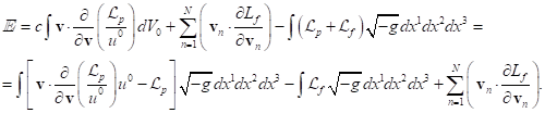
(2-31)
In (2-31), the energy ![]() is determined by the formula in which the
Lagrangian density
is determined by the formula in which the
Lagrangian density ![]() of the system is determined by the sum of two
terms, and the term
of the system is determined by the sum of two
terms, and the term ![]() directly depends on the four-currents
directly depends on the four-currents ![]() and
and ![]() , and
therefore
, and
therefore ![]() depends on the particle’s velocity
depends on the particle’s velocity ![]() .
.
Using for the components of
Lagrangian density expressions corresponding to vector fields in the form
![]() , (3-27)
, (3-27)
![]()
(4-28)
we can simplify expression (2-31)
for the energy of the system:
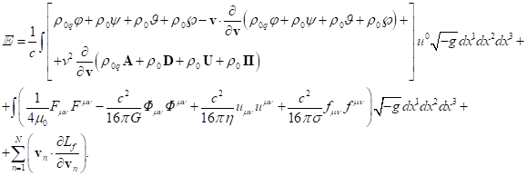
(5-36)
The momentum ![]() of the system in (1-45) is expressed by the
formula
of the system in (1-45) is expressed by the
formula
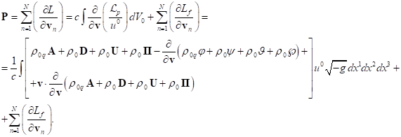
(6-37)
In this case, expressions (3-27) and
(4-28) are taken into account in (6-37).
The second method of calculating the
relativistic four-momentum ![]() of an arbitrary physical system involves
splitting
of an arbitrary physical system involves
splitting ![]() into two nonlocal four-vectors:
into two nonlocal four-vectors:
![]() .
(7-46)
.
(7-46)
To calculate the generalized
four-momentum ![]() in (7-46), it is necessary, under given
initial conditions, to determine the dependence of the metric tensor
in (7-46), it is necessary, under given
initial conditions, to determine the dependence of the metric tensor ![]() and its determinant
and its determinant ![]() on time and coordinates, and to find the time
component
on time and coordinates, and to find the time
component ![]() of the four-velocity
of the four-velocity ![]() of the particles of the system. In addition,
it is required to know the Lagrangian density
of the particles of the system. In addition,
it is required to know the Lagrangian density ![]() of the system so that the derivatives
of the system so that the derivatives ![]() can be calculated and then
can be calculated and then ![]() determined by integration over the moving
volume of the system:
determined by integration over the moving
volume of the system:
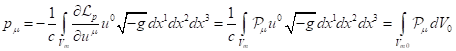 . (8-13)
Using ![]() (3-27), for
(3-27), for ![]() and its
components we have:
and its
components we have:
![]() . (9-38)
. (9-38)
![]() . (10-39)
. (10-39)
![]() . (11-40)
. (11-40)
Components of four-vector
![]()
in (7-46) with the use of (3-27) and
(4-28) are expressed by the formulas:
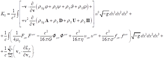
(12-47)
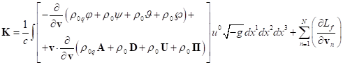 . (13-48)
Both of the methods presented above
for determining the relativistic four-momentum ![]() imply that first the equations for each field
acting in the system are solved, and the solutions to
the equation for the metric and the equation of motion of matter particles are
also found. After this, it becomes possible to determine the components of the
four-currents, metric tensor, four-potentials and field tensors required to
find
imply that first the equations for each field
acting in the system are solved, and the solutions to
the equation for the metric and the equation of motion of matter particles are
also found. After this, it becomes possible to determine the components of the
four-currents, metric tensor, four-potentials and field tensors required to
find ![]() .
.
Appendix B. Equations
(119-122)
Next, we use double numbering of formulas, in which the last digits
indicate the number of the formula in the text of the article.
We consider the stress-energy
tensor of the electromagnetic field with mixed indices:
![]() . (1-116)
. (1-116)
The time components of the
tensor ![]() (1-116) are expressed in terms of
the electric field strength
(1-116) are expressed in terms of
the electric field strength ![]() and magnetic field induction
and magnetic field induction ![]() in Cartesian coordinates as follows:
in Cartesian coordinates as follows:
![]() ,
, ![]() ,
,
![]() ,
, ![]() . (2-117)
. (2-117)
Inside the moving sphere in
the reference system ![]() , the components of
, the components of ![]() and
and ![]() are determined by the expressions
are determined by the expressions
![]() ,
, ![]() ,
, ![]() ,
,
![]() ,
, ![]() ,
, ![]() . (3-85)
. (3-85)
In the reference frame ![]() associated with the center of the sphere, there
is an electric field strength
associated with the center of the sphere, there
is an electric field strength ![]() inside the sphere, and the magnetic field
inside the sphere, and the magnetic field ![]() is zero due to the absence of internal currents.
Expressions (3-85) are obtained by transforming the electromagnetic field
tensor, containing components
is zero due to the absence of internal currents.
Expressions (3-85) are obtained by transforming the electromagnetic field
tensor, containing components ![]() and
and ![]() , from the reference system
, from the reference system ![]() to the
reference system
to the
reference system ![]() using Lorentz transformations.
using Lorentz transformations.
The electric field ![]() inside a sphere with charged particles in case
of the relativistic uniform system is expressed by the formula:
inside a sphere with charged particles in case
of the relativistic uniform system is expressed by the formula:
(4-81)
Substituting the components ![]() from (4-81) into (3-85), taking into account the
fact that in (4-81) there is the radius-vector
from (4-81) into (3-85), taking into account the
fact that in (4-81) there is the radius-vector ![]() , gives the following:
, gives the following:
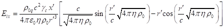 .
.
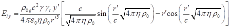 .
.
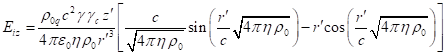 .
.
![]() ,
, 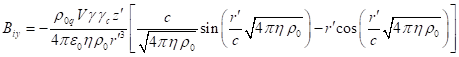 .
.
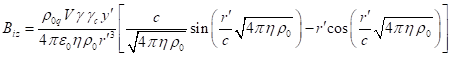 . (5)
. (5)
Taking into account the field
components (5), we find:
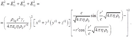
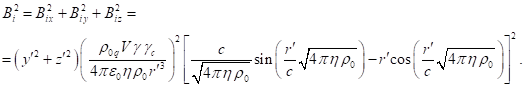
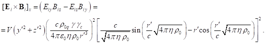
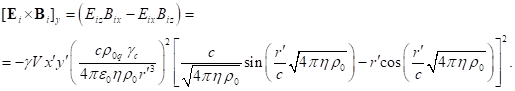
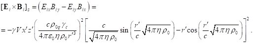
(6)
Substituting in (2-117) ![]() instead of
instead of ![]() and
and ![]() instead of
instead of ![]() , taking into account (6) and the relation
, taking into account (6) and the relation ![]() , we find:
, we find:
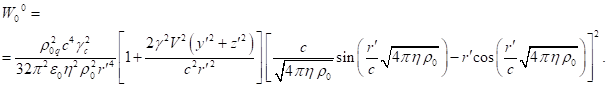
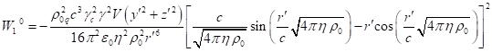 ,
,
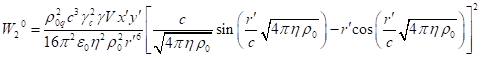 .
.
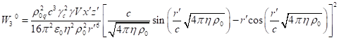 .
.
(7-119)
From the principle of least
action follow the equations of electromagnetic and gravitational fields,
acceleration fields and pressure fields. All these equations have the same
form, similar to Maxwell's equations. This is a consequence of the fact that these
fields are vector fields and have the same representation through the four-potentials
and tensors of these fields. As a result, the expression for the field tensors,
as well as for the stress-energy tensors for the electromagnetic field ![]() , for the gravitational field
, for the gravitational field ![]() , the acceleration field
, the acceleration field ![]() and the pressure field
and the pressure field ![]() turn out to be similar to each other and have
the same dependence on time and coordinates. To obtain the time components of
the stress-energy tensor
turn out to be similar to each other and have
the same dependence on time and coordinates. To obtain the time components of
the stress-energy tensor ![]() of the gravitational field, it is enough in
(7-119) to replace the charge density
of the gravitational field, it is enough in
(7-119) to replace the charge density ![]() with the mass density
with the mass density ![]() , and replace the electric constant
, and replace the electric constant ![]() with
with ![]() , as can be seen in (116):
, as can be seen in (116):
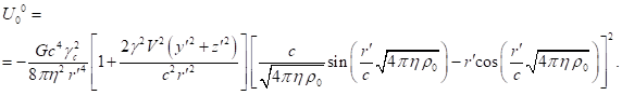
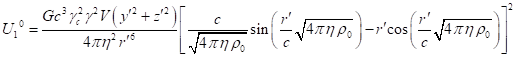 ,
,
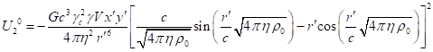 .
.
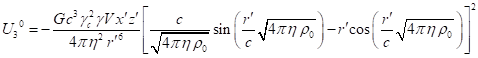 .
.
(8)
In the same way, we can find
the time components of the stress-energy tensors of the acceleration field and
the pressure field by replacing the charge density ![]() in (7-119) with the mass density
in (7-119) with the mass density ![]() , and replacing the electrical constant
, and replacing the electrical constant ![]() with
with ![]() and with
and with ![]() , respectively:
, respectively:
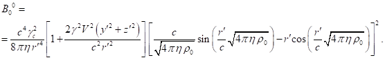
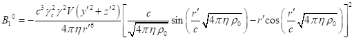 ,
,
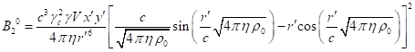 .
.
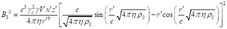 .
.
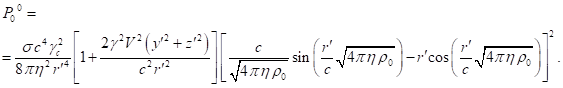
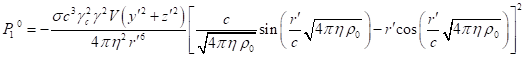 ,
,
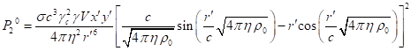 .
.
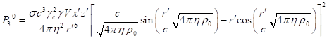 .
.
(9)
The stress-energy tensors in
(8-9) correspond to the expressions for the stress-energy tensors in Eq. (121)
of article.
The stress-energy tensor of a
physical system is obtained by summing the stress-energy tensors of all fields:
![]() . (10-115)
. (10-115)
Substituting (7-119), (8) and
(9) into (10-115) makes it possible to find the time components of the
stress-energy tensor:
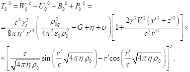
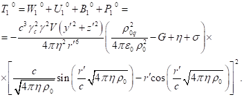

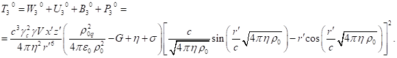
(11)
The equation of motion of
matter particles under the influence of fields is obtained from the principle
of least action. In the case of a relativistic uniform system, the equation of
motion implies the following relation for the field coefficients:
![]() .
(12-63)
.
(12-63)
If we substitute (12-63) into
(11), it becomes clear that in the matter of the moving sphere, which is a
relativistic uniform system, the time components ![]() ,
, ![]() ,
, ![]() and
and ![]() of stress-energy tensor of the system become equal
to zero.
of stress-energy tensor of the system become equal
to zero.
The integral vector is
determined by the expression:
![]() , (13-9)
, (13-9)
where index ![]() .
.
Since all
time components ![]() in the matter inside the moving sphere are equal
to zero according to (11) and (12-63), then the components of the integral
vector
in the matter inside the moving sphere are equal
to zero according to (11) and (12-63), then the components of the integral
vector ![]() in (13-9) become zero.
in (13-9) become zero.
Appendix C. List of symbols
![]() is four-potential of electromagnetic
field
is four-potential of electromagnetic
field
![]() is vector potential of electromagnetic
field
is vector potential of electromagnetic
field
![]() is radius of sphere
is radius of sphere
![]() is magnetic field induction
is magnetic field induction
![]() is stress-energy tensor of acceleration field with mixed indexes
is stress-energy tensor of acceleration field with mixed indexes
![]() is strength of pressure field
is strength of pressure field
![]() is speed of
light
is speed of
light
![]() is volume element in the form
of product of differentials of space coordinates
is volume element in the form
of product of differentials of space coordinates
![]() is four-potential of gravitational
field within the framework of covariant theory of gravitation
is four-potential of gravitational
field within the framework of covariant theory of gravitation
![]() is vector potential of gravitational
field
is vector potential of gravitational
field
![]() is electric field strength
is electric field strength
![]() is energy of a system
is energy of a system
![]() is energy of a system in reference frame
is energy of a system in reference frame ![]()
![]() is electric constant
is electric constant
![]() is four-force
is four-force
![]() is density of the four-force acting in a
unit element of the volume in which a typical particle with the number
is density of the four-force acting in a
unit element of the volume in which a typical particle with the number
![]() is located
is located
![]() is tensor of
electromagnetic field
is tensor of
electromagnetic field
![]() is tensor of
gravitational field
is tensor of
gravitational field
![]() is tensor of pressure
field
is tensor of pressure
field
![]() is scalar potential of electromagnetic
field
is scalar potential of electromagnetic
field
![]() is an angle coordinate of spherical coordinate system
is an angle coordinate of spherical coordinate system
![]() is gravitational constant
is gravitational constant
![]() or
or ![]() is metric tensor
is metric tensor
![]() is determinant of metric tensor
is determinant of metric tensor ![]()
![]() is metric tensor of Minkowski
spacetime
is metric tensor of Minkowski
spacetime
![]() is acceleration field coefficient
is acceleration field coefficient
![]() is strength of gravitational field
is strength of gravitational field
![]() denotes the
Lorentz factor of center of momentum of the moving sphere
denotes the
Lorentz factor of center of momentum of the moving sphere
![]() is the Lorentz factor of particles in
reference frame
is the Lorentz factor of particles in
reference frame ![]()
![]() is the Lorentz factor of particles at the
center of the sphere in reference frame
is the Lorentz factor of particles at the
center of the sphere in reference frame ![]()
![]() denotes the
Lorentz factor of a particle in reference frame
denotes the
Lorentz factor of a particle in reference frame ![]()
![]() is solenoidal vector of pressure field
is solenoidal vector of pressure field
![]() is integral vector in general theory of relativity
is integral vector in general theory of relativity
![]() is integral vector in covariant theory of
gravitation
is integral vector in covariant theory of
gravitation
![]() is auxiliary
four-dimensional quantity
is auxiliary
four-dimensional quantity
![]() is charge four-current
is charge four-current
![]() is mass four-current
is mass four-current
![]() is mass current density in reference frame
is mass current density in reference frame ![]()
![]() is charge current density in reference frame
is charge current density in reference frame ![]()
![]() or
or ![]() is field four-momentum
is field four-momentum
![]() is time component of
is time component of ![]() , which is associated with the energy in the term with the fields’ tensor
invariants
, which is associated with the energy in the term with the fields’ tensor
invariants
![]() is momentum of fields
is momentum of fields
![]() is Lagrangian
is Lagrangian
![]() represents the part of the
Lagrangian
represents the part of the
Lagrangian ![]() , that is
associated with tensor invariants
, that is
associated with tensor invariants
![]() denotes that part of the Lagrangian that is
associated with tensor invariants in the matter
denotes that part of the Lagrangian that is
associated with tensor invariants in the matter
![]() denotes that part of the Lagrangian that is
associated with tensor invariants outside the matter
denotes that part of the Lagrangian that is
associated with tensor invariants outside the matter
![]() represents the part of the
Lagrangian
represents the part of the
Lagrangian ![]() , which contains mass four-current
, which contains mass four-current ![]() and charge
four-current
and charge
four-current ![]()
![]() is Lagrangian inside the matter
is Lagrangian inside the matter
![]() is Lagrangian density
is Lagrangian density
![]() represents the
part of the Lagrangian density
represents the
part of the Lagrangian density ![]() , which contains tensor invariants
, which contains tensor invariants
![]() represents the
part of the Lagrangian density
represents the
part of the Lagrangian density ![]() , which contains mass four-current
, which contains mass four-current ![]() and charge
four-current
and charge
four-current ![]()
![]() is Lagrangian density inside the matter
is Lagrangian density inside the matter
![]() is cosmological constant
is cosmological constant
![]() is total mass of particles of
relativistic uniform system
is total mass of particles of
relativistic uniform system
![]() is gravitational mass of
relativistic uniform system
is gravitational mass of
relativistic uniform system
![]() is magnetic constant
is magnetic constant
![]() is total number of particles of a
physical system
is total number of particles of a
physical system
![]() is solenoidal vector of acceleration field
is solenoidal vector of acceleration field
![]() is current number of particle or volume
element
is current number of particle or volume
element
![]() is reference
frame of coordinate observer
is reference
frame of coordinate observer
![]() is reference
frame, associated with the center-of-momentum of moving sphere
is reference
frame, associated with the center-of-momentum of moving sphere
![]() is torsion field vector of gravitational field
is torsion field vector of gravitational field
![]() is three-dimensional relativistic
momentum of a system
is three-dimensional relativistic
momentum of a system
![]() is three-dimensional momentum of one
volume element or one particle
is three-dimensional momentum of one
volume element or one particle
![]() is relativistic momentum of particles
is relativistic momentum of particles
![]() or
or ![]() is
four-momentum of a system
is
four-momentum of a system
![]() is stress-energy tensor of pressure field with mixed indexes
is stress-energy tensor of pressure field with mixed indexes
![]() is
four-potential of pressure field
is
four-potential of pressure field
![]() is volume density of the generalized
four-momentum
is volume density of the generalized
four-momentum
![]() or
or ![]() is generalized four-momentum
is generalized four-momentum
![]() is time
component of the generalized four-momentum
is time
component of the generalized four-momentum
![]() is generalized momentum
is generalized momentum
![]() is vector potential of pressure field
is vector potential of pressure field
![]() is charge of a particle
is charge of a particle
![]() is total charge of relativistic uniform
system
is total charge of relativistic uniform
system
![]() is charge of moving sphere with particles
is charge of moving sphere with particles
![]() is an angle coordinate of spherical coordinate system
is an angle coordinate of spherical coordinate system
![]() is scalar potential of acceleration field
is scalar potential of acceleration field
![]() is scalar curvature
is scalar curvature
![]() is three-dimensional vector of position
is three-dimensional vector of position
![]() is radial
coordinate of spherical coordinate system
is radial
coordinate of spherical coordinate system
![]() is current
radius inside the sphere
is current
radius inside the sphere
![]() is mass density in particle’s comoving
reference frame
is mass density in particle’s comoving
reference frame
![]() is charge density in particle’s comoving
reference frame
is charge density in particle’s comoving
reference frame
![]() is scalar potential of pressure field
is scalar potential of pressure field
![]() is scalar potential of pressure field at the
center of the sphere in reference frame
is scalar potential of pressure field at the
center of the sphere in reference frame ![]()
![]() is action function
is action function
![]() is strength of acceleration field
is strength of acceleration field
![]() is Poynting vector
is Poynting vector
![]() is pressure field coefficient
is pressure field coefficient
![]() is coordinate time
is coordinate time
![]() is proper time
is proper time
![]() is stress-energy tensor
is stress-energy tensor
![]() is gravitational field pseudotensor
is gravitational field pseudotensor
![]() are time components of the stress-energy
tensor
are time components of the stress-energy
tensor
![]() are time components of the gravitational field pseudotensor
are time components of the gravitational field pseudotensor
![]() is vector potential of acceleration field
is vector potential of acceleration field
![]() is four-potential of acceleration field
is four-potential of acceleration field
![]() is stress-energy tensor of gravitational field with mixed indexes
is stress-energy tensor of gravitational field with mixed indexes
![]() or
or ![]() is four-velocity
is four-velocity
![]() is time component of four-velocity of
particle with the number
is time component of four-velocity of
particle with the number ![]()
![]() is tensor of acceleration
field
is tensor of acceleration
field
![]() is differential of volume element in comoving
reference frame
is differential of volume element in comoving
reference frame
![]() is volume occupied by matter
is volume occupied by matter
![]() is velocity of motion of the
system’s center of momentum
is velocity of motion of the
system’s center of momentum
![]() is velocity of a particle or
velocity of a volume element of matter in reference frame
is velocity of a particle or
velocity of a volume element of matter in reference frame ![]()
![]() is velocity of matter particle with
the current number
is velocity of matter particle with
the current number ![]()
![]() is velocity of typical particles in reference
frame
is velocity of typical particles in reference
frame ![]()
![]() is stress-energy tensor of electromagnetic field with mixed indexes
is stress-energy tensor of electromagnetic field with mixed indexes
![]() or
or ![]() is four-position
is four-position
![]() is scalar
potential of gravitational field
is scalar
potential of gravitational field
![]() is total field energy inside the matter, associated with tensor invariants
is total field energy inside the matter, associated with tensor invariants
![]() are Cartesian coordinates in reference frame
are Cartesian coordinates in reference frame ![]()
![]() are Cartesian coordinates in reference frame
are Cartesian coordinates in reference frame ![]()
References
1.
Landau L.D., Lifshitz E.M. Mechanics.
Vol. 1 (3rd ed.). (1976). Butterworth-Heinemann.
ISBN 978-0-7506-2896-9.
2.
Landau L.D., Lifshitz E.M. The Classical
Theory of Fields. (1951). Pergamon Press. ISBN
7-5062-4256-7.
3. Goldstein H., Poole C.P. and Safko J.L. Classical Mechanics (3rd ed.).
(2001). Addison-Wesley. p. 680. ISBN 9780201657029.
4.
M. Sharif, Tasnim
Fatima. Energy-Momentum Distribution: A Crucial Problem in General Relativity.
Int. J. Mod. Phys. A, Vol. 20, p. 4309 (2005). https://doi.org/10.1142/S0217751X05020793.
5.
Denisov V. I., Logunov A. A. The inertial mass defined in the general theory of relativity has no physical meaning. Theoretical and Mathematical
Physics, Vol. 51, Issue 2, pp. 421-426 (1982). http://dx.doi.org/10.1007/BF01036205.
6.
Denisov V. I., Logunov A. A. Does the general theory of relativity have a classical Newtonian limit? Theoretical and Mathematical Physics, Vol. 45, Issue 3, pp. 1035-1041 (1980). https://doi.org/10.1007%2FBF01016702.
7. Fedosin S.G. The covariant additive
integrals of motion in the theory of relativistic vector fields. Bulletin of
Pure and Applied Sciences, Vol. 37 D (Physics), No. 2, pp. 64-87 (2018). http://dx.doi.org/10.5958/2320-3218.2018.00013.1.
8.
Fedosin
S.G. The Principle of Least Action in Covariant
Theory of Gravitation. Hadronic Journal, Vol. 35, No. 1, pp. 35-70 (2012). http://dx.doi.org/10.5281/zenodo.889804.
9.
Dirac
P. A. M. General Theory of Relativity. (1975).
John Wiley & Sons Inc, quick presentation of the bare essentials of GTR. ISBN 978-0471215752.
10.
Khrapko, R. I. The Truth about the
Energy-Momentum Tensor
and Pseudotensor.
Gravitation and Cosmology, Vol. 20, No. 4, pp. 264-273 (2014). http://dx.doi.org/10.1134/S0202289314040082.
11. Fedosin S.G. About the cosmological constant, acceleration field, pressure
field and energy. Jordan Journal of Physics, Vol. 9, No. 1, pp. 1-30 (2016). http://dx.doi.org/10.5281/zenodo.889304.
12. Fedosin S.G. The Procedure of Finding the Stress-Energy Tensor and Equations of
Vector Field of Any Form. Advanced Studies in Theoretical Physics, Vol. 8, No.
18, pp. 771-779 (2014). http://dx.doi.org/10.12988/astp.2014.47101.
13. Fedosin S.G.
The concept of the general force vector field. OALib Journal, Vol. 3, pp. 1-15 (2016). http://dx.doi.org/10.4236/oalib.1102459.
14. Fedosin S.G.
Two components of the macroscopic general field. Reports in Advances of
Physical Sciences, Vol. 1, No. 2, 1750002 (2017). http://dx.doi.org/10.1142/S2424942417500025.
15. Fedosin S.G. The generalized
Poynting theorem for the general field and solution of the 4/3 problem.
International Frontier Science Letters, Vol. 14, pp. 19-40 (2019). https://doi.org/10.18052/www.scipress.com/IFSL.14.19.
16. Fedosin S.G.
Equations of Motion in the Theory of Relativistic Vector Fields. International
Letters of Chemistry, Physics and Astronomy, Vol. 83, pp. 12-30 (2019). https://doi.org/10.18052/www.scipress.com/ILCPA.83.12..
17. Fedosin S.G. Generalized
Four-momentum for Continuously Distributed Materials. Gazi University Journal
of Science, (2024). https://doi.org/10.35378/gujs.1231793.
18. Fock V.A. The
Theory of Space, Time and Gravitation. (1959). Pergamon Press, London..
19. Fedosin S.G.
Four-Dimensional Equation of Motion for Viscous Compressible and Charged Fluid
with Regard to the Acceleration Field, Pressure Field and Dissipation Field. International Journal of
Thermodynamics, Vol. 18, No. 1, pp. 13-24 (2015). https://doi.org/10.5541/ijot.5000034003.
20. Fedosin S.G. Energy and metric
gauging in the covariant theory of gravitation. Aksaray
University Journal of Science and Engineering, Vol. 2, Issue 2, pp. 127-143
(2018). http://dx.doi.org/10.29002/asujse.433947.
21. Fedosin S.G. Estimation of the physical parameters of planets and stars in the
gravitational equilibrium model. Canadian Journal of Physics, Vol. 94, No. 4,
pp. 370-379 (2016). http://dx.doi.org/10.1139/cjp-2015-0593.
22. Fedosin S.G.
The virial theorem and the kinetic energy of
particles of a macroscopic system in the general field concept. Continuum
Mechanics and Thermodynamics, Vol. 29, Issue 2, pp. 361-371 (2016). https://dx.doi.org/10.1007/s00161-016-0536-8.
23. Fedosin S.G. The Hamiltonian in Covariant Theory of Gravitation.
Advances in Natural Science, Vol. 5, No. 4, pp. 55-75 (2012). http://dx.doi.org/10.3968%2Fj.ans.1715787020120504.2023.
24. Fedosin S.G. The Gravitational Field in the Relativistic Uniform Model
within the Framework of the Covariant Theory of Gravitation. International
Letters of Chemistry, Physics and Astronomy, Vol. 78, pp. 39-50 (2018). http://dx.doi.org/10.18052/www.scipress.com/ILCPA.78.39.
25. Fedosin S.G. The Pioneer Anomaly in Covariant Theory of Gravitation. Canadian
Journal of Physics, Vol. 93, No. 11, pp. 1335-1342 (2015). http://dx.doi.org/10.1139/cjp-2015-0134.
26. Fedosin S.G. Relativistic Energy and Mass in the Weak Field Limit.
Jordan Journal of Physics. Vol. 8, No. 1, pp. 1-16 (2015). http://dx.doi.org/10.5281/zenodo.889210.
27. Searle G.F.C. On the steady motion
of an electrified ellipsoid. The Philosophical Magazine Series 5, 44 (269), 329-341 (1897). http://dx.doi.org/10.1088/1478-7814/15/1/323.
28. Fedosin S.G. 4/3 Problem for the Gravitational Field. Advances in Physics
Theories and Applications, Vol. 23, pp. 19-25 (2013). http://dx.doi.org/10.5281/zenodo.889383.
29.
Fedosin
S.G. The Integral Energy-Momentum 4-Vector and
Analysis of 4/3 Problem Based on the Pressure Field and Acceleration Field.
American Journal of Modern Physics. Vol. 3, No. 4, pp. 152-167 (2014). http://dx.doi.org/10.11648/j.ajmp.20140304.12.
Source: http://sergf.ru/wsen.htm