Continuum
Mechanics and Thermodynamics, Vol. 29, Issue 2, pp. 361-371 (2017). https://dx.doi.org/10.1007/s00161-016-0536-8.
The virial theorem and the
kinetic energy of particles of a macroscopic system in the general field
concept
Sergey
G. Fedosin
Sviazeva Str.
22-79, Perm, 614088, Perm Krai, Russian Federation
e-mail intelli@list.ru
The virial theorem is
considered for a system of randomly moving particles that are tightly bound to
each other by the gravitational and electromagnetic fields, acceleration field
and pressure field. The kinetic energy of the particles of this system is estimated
by three methods, and the ratio of the kinetic energy to the absolute value of
the energy of forces, binding the particles, is determined, which is
approximately equal to 0.6. For simple systems in classical mechanics, this
ratio equals 0.5. The difference between these ratios arises by the
consideration of the pressure field and acceleration field inside the bodies,
which make additional contribution to the acceleration of the particles. It is
found that the total time derivative of the system’s virial is not equal to
zero, as is assumed in classical mechanics for systems with potential fields.
This is due to the fact that although the partial time derivative of the virial
for stationary systems tends to zero, but in real bodies the virial also depends
on the coordinates and the convective derivative of the virial, as part of the
total time derivative inside the body, is not equal to zero. It is shown that
the convective derivative is also necessary for correct description of the
equations of motion of particles.
Keywords: virial
theorem; acceleration field; pressure field; general field;
kinetic energy.
1. Introduction
The virial theorem relates the
kinetic and potential energies of a stationary system in nonrelativistic
mechanics and is widely used in astrophysics for approximate evaluation of the
mass of large space systems, based on their sizes and the distribution of
velocities of individual objects [1]. The theorem statement in addition to the
gravitational field can also include other fields, such as the electromagnetic
field and the pressure field [2]. The relativistic modification of the theorem
takes into account the fact that the definition of momentum and kinetic energy
of each particle of the system also includes the corresponding Lorentz factor. In [3] by means of the virial
theorem the kinetic energy in a tensor form is associated at the microscopic
level with the stress tensor (Eshelby stress) in order to take into account the
pressure effects within the framework of classical physics and in [4] the
similar approach is used in variable-mass systems, where the fluxes of mass and
energy are taken into consideration.
In contrast to this we will
analyze the virial theorem for a system of closely interacting particles, which
are bound to each other by the gravitational and electromagnetic fields. In
this case we will use the concept of the vector pressure field, as well as the
concept of the acceleration vector field, in which the role of the
stress-energy tensor of matter is played by the stress- energy tensor of the
acceleration field [5, 6]. All these fields are parts of the general
field [7], which can be decomposed into two
main components. The source of the first component is the mass four-current ![]() , which
generates such vector fields as the gravitational field, acceleration field,
pressure field, dissipation field and macroscopic fields of strong and weak
interactions. The second component of the general field is the electromagnetic
field, the source of which is the charge four-current
, which
generates such vector fields as the gravitational field, acceleration field,
pressure field, dissipation field and macroscopic fields of strong and weak
interactions. The second component of the general field is the electromagnetic
field, the source of which is the charge four-current ![]() .
.
In the derivation of the
virial theorem it is generally assumed that the time derivative of the virial
of the system, averaged over time, tends to zero. By direct calculation we will
show that in our model this is not exactly so and will provide our explanation
for this state of things, taking into account the relation between the general
field components.
2. The virial theorem
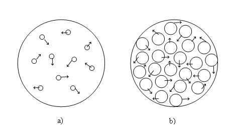
Suppose there is a bounded system of a number of
randomly moving small particles, which has a spherical shape and is in
equilibrium under the action of the proper gravitational and electromagnetic
fields, acceleration field and pressure field. If the spaces between the
particles are small, as in a liquid, it can be assumed that the matter inside
this sphere is distributed uniformly. We studied such a physical system in [8], where the
field strengths, potentials and energies of all the four fields were first
defined in the framework of the relativistic uniform model.
Let us place the origin of the coordinate system at
the center of the sphere and apply the virial theorem to this system of
particles and fields. This system is stable, the particles are bound by the
forces arising from the action of the fields, and therefore the conditions of
the theorem are satisfied. The virial theorem in a relativistic form can be written as follows:
![]() ,
(1)
,
(1)
where ![]() is the virial as a certain scalar function; the symbol
is the virial as a certain scalar function; the symbol ![]() denotes averaging over a sufficiently large period of time;
denotes averaging over a sufficiently large period of time; ![]() is a quantity that in the limit of low velocities tends to the total kinetic energy of all
is a quantity that in the limit of low velocities tends to the total kinetic energy of all ![]() particles of the system;
particles of the system; ![]() is the Lorentz factor of the
is the Lorentz factor of the ![]() -th particle with the mass
-th particle with the mass ![]() and velocity
and velocity ![]() ; the vectors
; the vectors ![]() and
and ![]() denote the radius-vector and relativistic
momentum of the
denote the radius-vector and relativistic
momentum of the ![]() -th particle,
-th particle, ![]() is the total force, acting on the
is the total force, acting on the ![]() -th particle.
-th particle.
In order to
pass on to the virial theorem in its classic form, it is sufficient to equate
in (1) the Lorentz factors of all the particles to unity, that is to assume ![]() .
.
Figure 1
shows that in contrast to the discrete distribution of particles, in order to
use the continuous distribution approximation it is necessary to detect in the
matter of the system under consideration the particles of such a size, that the
gaps between them would be close to zero, and to assume that the sphere’s
volume is made up of the volumes of these particles. Each particle of this type
occupies a certain representative volume element of the system, which is
sufficient for the correct description of the typical properties of particles
and acting fields.
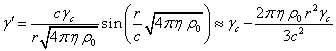
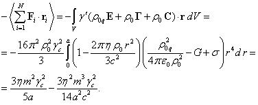
Let us first calculate the value ![]() in the left-hand side of (1), substituting
in the left-hand side of (1), substituting ![]() with
with ![]() and the sum over all the particles with the
integral over the volume of the fixed sphere. The value
and the sum over all the particles with the
integral over the volume of the fixed sphere. The value ![]() is the mass density in the reference frames
associated with the particles,
is the mass density in the reference frames
associated with the particles, ![]() is the Lorentz factor of the moving particles,
the product
is the Lorentz factor of the moving particles,
the product ![]() gives the mass density of the particles from
the point of view of the observer, stationary with respect to the sphere, and
the volume element
gives the mass density of the particles from
the point of view of the observer, stationary with respect to the sphere, and
the volume element ![]() inside the sphere corresponds to the volume of
a particle from the point of view of this observer. We can assume that the
total volume of the particles at rest is greater than the volume of the sphere,
but because of the motion the volume of each particle decreases due to the
length contraction effect of the special theory of relativity.
inside the sphere corresponds to the volume of
a particle from the point of view of this observer. We can assume that the
total volume of the particles at rest is greater than the volume of the sphere,
but because of the motion the volume of each particle decreases due to the
length contraction effect of the special theory of relativity.
Actually, to apply the relativistic formulas
correctly, the volume of any moving spherical particle is modeled by the
so-called Heaviside ellipsoid, which has been first mentioned in [9]. It turns
out that the volume of this ellipsoid is smaller than the volume of the
particle under consideration in the reference frame associated with the
particle by the value of the Lorentz factor. All this leads to the fact that
the total volume of the particles moving inside the sphere becomes equal to the
volume of the sphere.
The same can be said in other words. If we divide
the system’s matter into separate independently moving particles, as is shown
in Fig. 1 b, then the sum of the volumes of Heaviside ellipsoids of all
particles should be equal to the volume of the sphere and the sum of the proper
volumes of these particles, respectively, will be greater than the volume of
the sphere.
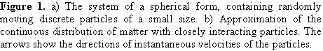
According to [8], the Lorentz factor ![]() for the particles inside the fixed sphere is a
function of the current radius
for the particles inside the fixed sphere is a
function of the current radius ![]() :
:
 , (2)
, (2)
where ![]() is the speed of light,
is the speed of light, ![]() is the acceleration field coefficient,
is the acceleration field coefficient, ![]() is the Lorentz factor for the
velocities
is the Lorentz factor for the
velocities ![]() of the particles at the center of the sphere, and in
view of the smallness of the argument the sine can be expanded into
second-order terms.
of the particles at the center of the sphere, and in
view of the smallness of the argument the sine can be expanded into
second-order terms.
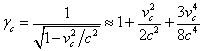
The second expansion term in (2) can be
represented as follows:
![]() ,
,
where the expression ![]() gives an estimate of the mass contained inside
the current radius
gives an estimate of the mass contained inside
the current radius ![]() of the sphere,
of the sphere, ![]() is the gravitational potential created by the
spherical mass
is the gravitational potential created by the
spherical mass ![]() on the radius
on the radius ![]() .
.
In cosmic bodies held by their own
gravitation the acceleration field coefficient ![]() differs from
the gravitational constant
differs from
the gravitational constant ![]() only by a small
numerical factor of the order of unity, and the Lorentz factor
only by a small
numerical factor of the order of unity, and the Lorentz factor ![]() is only
slightly greater than unity for the majority of bodies. As a result, the second expansion term in (2)
can be considered as the ratio of the absolute value of the average
gravitational potential inside the body to the square of the speed of light.
This ratio is small and starts to increase significantly only in white dwarfs
and neutron stars. Despite the smallness of the second term, it is absolutely
essential for justification of our relativistic approach. Indeed, let us square the equation for
is only
slightly greater than unity for the majority of bodies. As a result, the second expansion term in (2)
can be considered as the ratio of the absolute value of the average
gravitational potential inside the body to the square of the speed of light.
This ratio is small and starts to increase significantly only in white dwarfs
and neutron stars. Despite the smallness of the second term, it is absolutely
essential for justification of our relativistic approach. Indeed, let us square the equation for ![]() in (2) and we will obtain approximately the following:
in (2) and we will obtain approximately the following:
![]() .
(3)
.
(3)
The velocity ![]() of the random motion of particles inside the
sphere is a function of the current radius
of the random motion of particles inside the
sphere is a function of the current radius ![]() only. In this case, as the volume element we
can take the volume of the thin spherical layer:
only. In this case, as the volume element we
can take the volume of the thin spherical layer: ![]() . Equating
. Equating ![]() and
and ![]() from (1) to
from (1) to ![]() in (2) and
in (2) and ![]() in (3), respectively, and substituting
in (3), respectively, and substituting ![]() with
with ![]() , for
, for ![]() we obtain the following:
we obtain the following:
 (4)
(4)
Here, the mass ![]() ,
which has auxiliary character, is equal
to the product of the density
,
which has auxiliary character, is equal
to the product of the density ![]() by the volume of the sphere, with the radius
of the sphere equal to
by the volume of the sphere, with the radius
of the sphere equal to ![]() .
.
By analogy with [5], the equation of motion of the particles can
be written as follows:
![]() . (5)
. (5)
A distinctive feature of this equation as opposed
to the equation of motion in [5] is that it is written not for a particular
physical particle but for a representative particle, which behaves as a certain
typical particle averaged with respect to all parameters. This is indicated by
the fact that ![]() as the Lorentz factor and the velocity
as the Lorentz factor and the velocity ![]() are used, which are found from the equations
of the acceleration field, while for a physical particle usually its
instantaneous velocity and the Lorentz factor, corresponding to this velocity,
are taken into account. We can assume that Eq. (5) is the result of averaging
of the equations of motion for a certain ensemble of physical particles, so
that a typical equation of motion for typical particles is obtained.
are used, which are found from the equations
of the acceleration field, while for a physical particle usually its
instantaneous velocity and the Lorentz factor, corresponding to this velocity,
are taken into account. We can assume that Eq. (5) is the result of averaging
of the equations of motion for a certain ensemble of physical particles, so
that a typical equation of motion for typical particles is obtained.
The right-hand side of (5) represents the total density of the force acting on a typical particle inside the sphere. This force density must be
multiplied by the radius ![]() , where this
particle is located, and then integrated over the entire volume of the sphere
in order to calculate the second term in the right-hand side of (1). The force
density in (5) should also be multiplied by
, where this
particle is located, and then integrated over the entire volume of the sphere
in order to calculate the second term in the right-hand side of (1). The force
density in (5) should also be multiplied by ![]() in order to obtain the product
in order to obtain the product ![]() , which in
view of the expression
, which in
view of the expression ![]() after integration over the volume will be
equivalent to the expression for the force
after integration over the volume will be
equivalent to the expression for the force ![]() .
.
We will take into account that the magnetic
induction vector ![]() , the
solenoidal vector (the torsion field)
, the
solenoidal vector (the torsion field) ![]() of the gravitational field and the solenoidal
vector
of the gravitational field and the solenoidal
vector ![]() of the pressure field inside the fixed sphere
are equal to zero due to the random motion of particles. In this case,
according to [8] we have the following:
of the pressure field inside the fixed sphere
are equal to zero due to the random motion of particles. In this case,
according to [8] we have the following:
![]() ,
, ![]() ,
, ![]() ,
,
and we can write:
 (6)
(6)
In (5) and (6), ![]() ,
, ![]() and
and ![]() are the field strengths of the electric field,
the gravitational field and the pressure field, respectively,
are the field strengths of the electric field,
the gravitational field and the pressure field, respectively, ![]() is the charge density of the particles in the
reference frames associated with the particles,
is the charge density of the particles in the
reference frames associated with the particles, ![]() is the
vacuum permittivity,
is the
vacuum permittivity, ![]() is the gravitational constant, and
is the gravitational constant, and ![]() is the pressure field coefficient. Besides,
the correlation between the field coefficients was used, which had been
obtained in [10] using the equations of motion:
is the pressure field coefficient. Besides,
the correlation between the field coefficients was used, which had been
obtained in [10] using the equations of motion:
![]() .
(7)
.
(7)
In order to arrive at (7), it will suffice to
express the left-hand side of (5) in terms of the field strength ![]() and the solenoidal vector
and the solenoidal vector ![]() of the acceleration field in the framework of
the special theory of relativity [5]:
of the acceleration field in the framework of
the special theory of relativity [5]:
![]() .
.
Next we should take into account the equality of
the solenoidal vector ![]() and the vector potential
and the vector potential ![]() to zero in the system under consideration, as
well as the expression for the scalar potential of the acceleration field in
the form
to zero in the system under consideration, as
well as the expression for the scalar potential of the acceleration field in
the form ![]() . Then the
field strength of the acceleration field in view of (2) is given by the
formula:
. Then the
field strength of the acceleration field in view of (2) is given by the
formula:
![]() .
.
Using further in (5) the
expressions given above for ![]() ,
, ![]() and
and ![]() , we arrive at (7). Actually relation (7) for the fields’ coefficients is
the consequence of the local balance of the forces and energies, associated
with the fields, acting on the particles.
, we arrive at (7). Actually relation (7) for the fields’ coefficients is
the consequence of the local balance of the forces and energies, associated
with the fields, acting on the particles.
The virial ![]() contains the scalar vector products of the
form
contains the scalar vector products of the
form ![]() . In these
products we will substitute the particles’ velocities
. In these
products we will substitute the particles’ velocities ![]() with the averaged velocities of random motion
with the averaged velocities of random motion ![]() , which
depend on the current radius, according to (3). Then we will assume that
, which
depend on the current radius, according to (3). Then we will assume that ![]() , where
, where ![]() denotes the averaged velocity component,
directed along the radius, and
denotes the averaged velocity component,
directed along the radius, and ![]() is the averaged velocity component,
perpendicular to the current radius. Then for the particles inside the sphere
is the averaged velocity component,
perpendicular to the current radius. Then for the particles inside the sphere ![]() . Based on
statistical considerations, it follows that:
. Based on
statistical considerations, it follows that:
![]() .
(8)
.
(8)
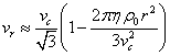
For the dependence of the magnitude of the radial
velocity component on the current radius we can write in the first
approximation:
![]() . (9)
. (9)
Thus, we assume that the dependence of the radial
velocity component ![]() on the radius due to its form can be represented
similarly to the squared velocity
on the radius due to its form can be represented
similarly to the squared velocity ![]() in (3). To prove this assumption we will
square expression (9) and substitute it in (8) instead of
in (3). To prove this assumption we will
square expression (9) and substitute it in (8) instead of ![]() , and then
we will find the value of
, and then
we will find the value of ![]() and compare it with (3).
and compare it with (3).
This allows us to estimate the coefficients ![]() and
and ![]() and to rewrite (9) as follows:
and to rewrite (9) as follows:
 .
(10)
.
(10)
Therefore, for the product of vectors in the
virial we will have approximately the following:
![]() . (11)
. (11)
The time derivative of the virial in (1) should
be regarded as the material derivative:
![]() ,
(12)
,
(12)
besides, in our case the virial does not depend
on time and ![]() .
.
We can calculate the product ![]() ,
substituting in it
,
substituting in it ![]() with
with ![]() , since the
virial
, since the
virial ![]() depends only on the radius, and the virial
gradient
depends only on the radius, and the virial
gradient ![]() is directed along the radius. Taking into
account (11), (2) for the Lorentz factor, (10) for the magnitude of the radial
velocity
is directed along the radius. Taking into
account (11), (2) for the Lorentz factor, (10) for the magnitude of the radial
velocity ![]() , as well
the expression
, as well
the expression ![]() used instead of the mass
used instead of the mass ![]() , which before
that must be taken outside the gradient sign, we find:
, which before
that must be taken outside the gradient sign, we find:

(13)
Substituting (13) into (12), provided that ![]() ,
finding
,
finding ![]() and using it in (1), in view of (4) and (6) we
obtain an approximate relation:
and using it in (1), in view of (4) and (6) we
obtain an approximate relation:
![]() .
.
Considering this relation as a quadratic equation
for ![]() and solving this equation, we arrive at the
following:
and solving this equation, we arrive at the
following:
![]() . (14)
. (14)
With ![]() and in view of (14), Eq. (3) gives an expression for the squared
velocity of the particles near the sphere’s surface:
and in view of (14), Eq. (3) gives an expression for the squared
velocity of the particles near the sphere’s surface:
![]() .
.
Hence it follows that ![]() .
This means that as a consequence of the virial theorem, the square of the velocity
of particles
.
This means that as a consequence of the virial theorem, the square of the velocity
of particles ![]() in the center is about 4 times greater than
the square of the velocity of particles
in the center is about 4 times greater than
the square of the velocity of particles ![]() near the surface of the sphere. Since the
squared velocities are proportional to the kinetic energy and temperature,
then, under condition of the constant mass density
near the surface of the sphere. Since the
squared velocities are proportional to the kinetic energy and temperature,
then, under condition of the constant mass density ![]() in the considered idealized system, the
temperatures at the center and near the surface must
not differ more than 4.1 times. Among the real objects, the density of which does
not change much with the current radius, we can take Bok globules. Their
typical radius is 0.35 parsecs, the mass is 11 Solar masses, and the recorded
temperature of dust in some globules may reach 26 K [11]. In [10], based on the equations of motion of
particles, the kinetic temperature of the particles near the surface of a
globule was estimated:
in the considered idealized system, the
temperatures at the center and near the surface must
not differ more than 4.1 times. Among the real objects, the density of which does
not change much with the current radius, we can take Bok globules. Their
typical radius is 0.35 parsecs, the mass is 11 Solar masses, and the recorded
temperature of dust in some globules may reach 26 K [11]. In [10], based on the equations of motion of
particles, the kinetic temperature of the particles near the surface of a
globule was estimated: ![]() K. If we assume that
K. If we assume that ![]() , then the central temperature is
, then the central temperature is ![]() K,
which is close enough to observations.
K,
which is close enough to observations.
Using (14) for substituting in (4) and in (13) in
view of (12):
![]() ,
, ![]() . (15)
. (15)
Expressions (15) and (6) agree well with the
virial theorem (1) in the approximation under consideration. In addition, in
(15) we can see that the time derivative of the virial ![]() after averaging is not equal to zero, as is
usually assumed in classical mechanics. From (15) and (6) the relation follows:
after averaging is not equal to zero, as is
usually assumed in classical mechanics. From (15) and (6) the relation follows:
![]() .
(16)
.
(16)
Meanwhile, in the conventional interpretation of
the virial theorem the kinetic energy of the system of particles must be two
times less than the energy, associated with the forces, holding the particles:
![]() , (17)
, (17)
If we substitute (14) in (10), we will obtain the
following:
![]() .
.
If we take into account (8), then for the
velocities’ amplitudes we can write ![]() . We
see that inside the sphere there are radial gradients both of the radial
component
. We
see that inside the sphere there are radial gradients both of the radial
component ![]() and of the velocity component
and of the velocity component ![]() perpendicular to the radius, and also there is
a gradient of the squared velocity of particles
perpendicular to the radius, and also there is
a gradient of the squared velocity of particles ![]() in (3), while
in (3), while ![]() . The
velocity
. The
velocity ![]() leads to a certain centripetal acceleration
directed along the radius. Due to this as well as due to the radial action of
the pressure field and the electric field the acceleration arises, which counteracts
the gravitational acceleration and leads to a noticeable difference between
(16) and (17).
leads to a certain centripetal acceleration
directed along the radius. Due to this as well as due to the radial action of
the pressure field and the electric field the acceleration arises, which counteracts
the gravitational acceleration and leads to a noticeable difference between
(16) and (17).
The difference of (16) from the classical case
(17) is caused by the fact that we take into account not the usual uniformity
of mass and charge in the reference frame of the sphere, but the relativistic
uniformity, when the mass and charge densities are constant in their own
reference frames, associated with individual particles. This leads to a change
in the values of the field strengths of all the fields inside the sphere and of
the field strengths of the gravitational and electromagnetic fields outside the
sphere, as well as to a change in accelerations from the action of respective
forces.
It follows from (16) that at the constant potential energy (6), associated
with the forces holding the particles of the system, the kinetic energy of
motion must be greater than in (17) by a value of about 20%. As the density
non-uniformity inside the system increases, the difference between (16) and
(17) may change even more.
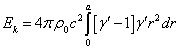
3. The kinetic energy: standard definition
Within the framework of the
special theory of relativity, the kinetic energy of a particle is calculated as
the difference between the relativistic energy of a moving particle and the energy
of the particle at rest. For a system of ![]() particles we obtain the following:
particles we obtain the following:
![]() .
(18)
.
(18)
Let us use in (18) instead of ![]() the Lorentz factor
the Lorentz factor ![]() from (2), and replace the mass
from (2), and replace the mass ![]() by
by ![]() and the sum over all the particles by the
integral over the volume of a fixed sphere:
and the sum over all the particles by the
integral over the volume of a fixed sphere:
 .
.
 (19)
(19)
Let us substitute the Lorentz
factor in (19):
 ,
, ![]() .
.
(20)
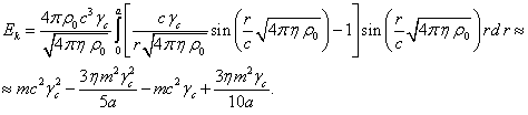
Substituting ![]() from (14) in (20) we find the approximate
expression for the kinetic energy:
from (14) in (20) we find the approximate
expression for the kinetic energy:
![]() . (21)
. (21)
Within the limit of low
velocities, with an accuracy up to the terms of the second order of smallness,
the expression for ![]() in (21) coincides with the energy
in (21) coincides with the energy ![]() in (15),
which proves our calculations of the kinetic energy based on the relativistic
energy definition and the energy estimate based on the virial theorem.
in (15),
which proves our calculations of the kinetic energy based on the relativistic
energy definition and the energy estimate based on the virial theorem.
Note that when we determine ![]() we use the Lorentz factor
we use the Lorentz factor ![]() from (2), which is found through the
acceleration field of the particles inside the sphere, instead of the Lorentz
factor of individual particles moving randomly. Thus, the kinetic energy
from (2), which is found through the
acceleration field of the particles inside the sphere, instead of the Lorentz
factor of individual particles moving randomly. Thus, the kinetic energy ![]() in (19) and (21) is obtained as a certain
approximation to the actual kinetic energy of the particles.
in (19) and (21) is obtained as a certain
approximation to the actual kinetic energy of the particles.
4. The energy of motion
In [5] we gave the definition of the energy of the
particles’ motion using the generalized 3-momenta ![]() of the system’s particles:
of the system’s particles:
![]() ,
,
where ![]() is the 3-vector of velocity of the particle
with the number
is the 3-vector of velocity of the particle
with the number ![]() ;
; ![]() specifies the number of particles in
the system; and the generalized momentum of each particle is expressed in terms
of the particle Lagrangian
specifies the number of particles in
the system; and the generalized momentum of each particle is expressed in terms
of the particle Lagrangian ![]() according to the formula:
according to the formula: ![]() .
.
This energy can also be
written as the half-sum of the Hamiltonian ![]() and the Lagrangian
and the Lagrangian ![]() of the system of particles and four fields:
of the system of particles and four fields:
![]()
(22)
where
![]() ,
, ![]() ,
, ![]() and
and ![]() denote the vector potentials of the
acceleration field, gravitational field, electromagnetic field and pressure
field, respectively;
denote the vector potentials of the
acceleration field, gravitational field, electromagnetic field and pressure
field, respectively; ![]() is the time component of the particle’s
four-velocity;
is the time component of the particle’s
four-velocity; ![]() is the determinant of the metric tensor;
is the determinant of the metric tensor; ![]() is the product of the spatial coordinates’
differentials.
is the product of the spatial coordinates’
differentials.
The
Hamiltonian ![]() and the Lagrangian
and the Lagrangian ![]() of the system, which are present in (22), were
determined in [5] in a covariant way for the curved spacetime, while the
expression for the conserved over time relativistic energy of an arbitrary
isolated system coincides with the expression for the Hamiltonian
of the system, which are present in (22), were
determined in [5] in a covariant way for the curved spacetime, while the
expression for the conserved over time relativistic energy of an arbitrary
isolated system coincides with the expression for the Hamiltonian ![]() . It should
be noted that the energy of motion
. It should
be noted that the energy of motion ![]() does not contain any scalar curvature or the
cosmological constant and thus does not depend on the method of gauging the
relativistic energy of the system.
does not contain any scalar curvature or the
cosmological constant and thus does not depend on the method of gauging the
relativistic energy of the system.
Within the framework of the special theory of relativity for the particles inside a fixed sphere we can assume that ![]() . In the random motion of particles
the total vector potentials of all the fields, averaged over the entire set of
particles, are equal to zero. However, the vector potentials of each individual
particle are equal to zero only at rest, but in case of motion they are
proportional to the particle velocity and to the scalar potentials of the
proper fields of particles and inversely proportional to the squared speed of
light. This follows from the definition of the four-potential of each field [6], as well as from the solution of the wave
equation for the vector potential of the corresponding field at a constant
velocity of the particle’s motion.
. In the random motion of particles
the total vector potentials of all the fields, averaged over the entire set of
particles, are equal to zero. However, the vector potentials of each individual
particle are equal to zero only at rest, but in case of motion they are
proportional to the particle velocity and to the scalar potentials of the
proper fields of particles and inversely proportional to the squared speed of
light. This follows from the definition of the four-potential of each field [6], as well as from the solution of the wave
equation for the vector potential of the corresponding field at a constant
velocity of the particle’s motion.
It
should be noted that in (22) integration is done over the volume of each
particle separately and then summation is performed over all the particles. In
integration over the volume of one particle, the velocity of this particle is
considered as a constant and can be taken out of the integral sign. As a
result, we can rewrite (22) as follows:
![]() . (23)
. (23)
In
(23) ![]() ,
, ![]() ,
, ![]() and
and ![]() denote the proper scalar potentials of the
moving particles for the acceleration field, gravitational field,
electromagnetic field and pressure field, respectively; the quantity
denote the proper scalar potentials of the
moving particles for the acceleration field, gravitational field,
electromagnetic field and pressure field, respectively; the quantity ![]() is the Lorentz factor of particles according
to (2). As it was shown in [12], from the
gauge of the system energy using the cosmological constant
is the Lorentz factor of particles according
to (2). As it was shown in [12], from the
gauge of the system energy using the cosmological constant ![]() the following expression was obtained:
the following expression was obtained:
![]() ,
,
where ![]() ;
;
![]() is the constant of the order of
unity, which is included as a multiplier in the equation for the metric;
is the constant of the order of
unity, which is included as a multiplier in the equation for the metric;
![]() is the gauge mass as the
total mass of the system’s particles, removed from the system to infinity and being there at
rest, taking into account the energies of particles in the potentials of the
proper fields, but neglecting the field energies as such.
is the gauge mass as the
total mass of the system’s particles, removed from the system to infinity and being there at
rest, taking into account the energies of particles in the potentials of the
proper fields, but neglecting the field energies as such.
From (23) we then obtain the
following:
![]() .
(24)
.
(24)
Comparison with the expression
![]() from (1) shows that
from (1) shows that ![]() tends to the energy
tends to the energy ![]() only in the limit of low velocities, where we
can neglect the Lorentz factors of the particles.
only in the limit of low velocities, where we
can neglect the Lorentz factors of the particles.
As a first approximation, in
(24) we will replace the mass ![]() by
by ![]() , the
squared velocity
, the
squared velocity ![]() by
by ![]() from (3), use
from (3), use ![]() from (2), and represent the sum over all the
particles as the integral over the volume of the fixed sphere:
from (2), and represent the sum over all the
particles as the integral over the volume of the fixed sphere:
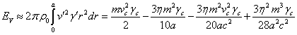 .
.
If we equate the obtained integral for ![]() to the first integral for
to the first integral for ![]() from (19), it gives the relation for the
Lorentz factor of the form
from (19), it gives the relation for the
Lorentz factor of the form ![]() , which can
be considered valid in the first-order approximation. The difference between
, which can
be considered valid in the first-order approximation. The difference between ![]() and
and ![]() in (20) occurs in the terms containing the
squared speed of light in the denominator. Hence it follows that the energy of
motion (22), determined with the help of the generalized momenta and the proper
fields of particles, is close enough to the kinetic energy of particles
in (20) occurs in the terms containing the
squared speed of light in the denominator. Hence it follows that the energy of
motion (22), determined with the help of the generalized momenta and the proper
fields of particles, is close enough to the kinetic energy of particles ![]() , which is
found with the help of the distribution of particles in the acceleration field.
, which is
found with the help of the distribution of particles in the acceleration field.
5. The analysis of the equation
of motion
We will transform the equation
of motion of typical particles (5) multiplying it scalarly by the vector quantity ![]() :
:
![]() . (25)
. (25)
We will calculate the term on
the left-hand side of this equation, substituting the Lorentz factor ![]() from (2), and the value of
from (2), and the value of ![]() from (3). In this case the total time
derivative will be regarded as the material derivative, in which in the
convective derivative the velocity
from (3). In this case the total time
derivative will be regarded as the material derivative, in which in the
convective derivative the velocity ![]() with amplitude (10) can be used instead of the
velocity
with amplitude (10) can be used instead of the
velocity ![]() . Neglecting
the small terms with the square of the speed of light, we find:
. Neglecting
the small terms with the square of the speed of light, we find:
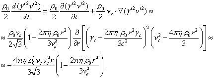 (26)
(26)
Since the system under
consideration is stationary, then the partial time derivative ![]() in (26) is equal to zero. The need to use the material derivative in (25)
and (26) is due to the fact that the product
in (26) is equal to zero. The need to use the material derivative in (25)
and (26) is due to the fact that the product ![]() is the function of the spatial coordinates,
but is time-independent. However, relation (25) must be valid for all reference
frames, including the reference frame moving radially at the velocity
is the function of the spatial coordinates,
but is time-independent. However, relation (25) must be valid for all reference
frames, including the reference frame moving radially at the velocity ![]() . In this
reference frame the gradient
. In this
reference frame the gradient ![]() is other than zero, and then the derivative
is other than zero, and then the derivative ![]() is not equal zero.
is not equal zero.
We will now calculate the
right-hand side of (25), substituting there the expressions for the field
strengths ![]() ,
, ![]() and
and ![]() , which were
used in (6). In this case we will take into account that all the forces are
directed along the radius and therefore the velocity
, which were
used in (6). In this case we will take into account that all the forces are
directed along the radius and therefore the velocity ![]() can be replaced with
can be replaced with ![]() :
:
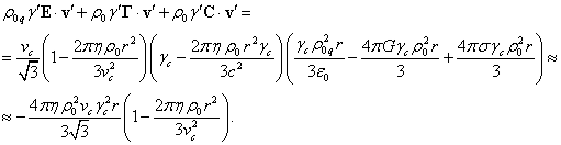 (27)
(27)
In (27), relation (7) for the
field coefficients was used. Within the accuracy of the assumptions made for the
velocities and the Lorentz factor, expressions (26) and (27) coincide,
illustrating the validity of equation of motion (5) for the averaged velocities
of particles inside the sphere and the need to use the material derivative.
6. Conclusion
In (1) we presented the
relativistic expression of the virial theorem and then calculated each term of
this expression. In (10) we obtained the approximate dependence of the
amplitude of the radial component of the particles’ velocity on the current
radius, which is associated with the acceleration field acting in the system.
For a stationary system the partial time derivative of the virial vanishes, and
it becomes important to take into account the dependence of the virial on the
space coordinates in the expression for the material derivative (12). As a
consequence of the virial theorem, it becomes possible to estimate the velocity
of particles at the center of the system in relation (14), and then to express
the kinetic energy in terms of the acceleration field coefficient in (15).
In (16) we obtained the
coefficient, relating the kinetic energy of particles and the energy of the
forces acting on them, which is approximately equal to 0.6. Taking into account
the pressure field and the acceleration field leads to 20 % difference between
this coefficient and the standard value of 0.5 in (17) for systems without
pressure.
From the physical standpoint,
the discrepancy between these coefficients arises as a result of different
interpretations of the concept of a homogeneous system: in classical mechanics
the body mass density at each point is assumed to be the same in the reference
frame, associated with the body, but in relativistic mechanics the mass density
must be the same for each particle of the body, regardless of its motion, i.e.,
to be invariant under Lorentz transformations. The invariant mass density of
the body’s particle is the density, which is found in the reference frame
associated with this particle. As a result, the particles, that move at the
center of the body and have an increased velocity, have a greater mass density
in the reference frame, associated with the body, which leads to the radial
gradient of density and other variables inside the body in question and to
correction of the virial theorem.
To check our calculations, the
kinetic energy was calculated in (21) in another way, as a difference between
the energies of the moving particles and the particles at rest. In (24) we also
estimated the energy of the particles’ motion using the generalized momenta and
the proper fields of the particles, which turned out to be almost exactly equal
to the kinetic energy.
In (26) and (27) we also
checked whether equation of motion (5) is precisely satisfied, when the
expression for the radial velocity (10) is used for the case, in which not the
velocity of a specific particle is substituted in the equation of motion but
the averaged random velocity of particles as a function of the radius. It turns
out that in this case the time derivative in the equation of motion should be
regarded as material derivative, which takes into account not only the change
in the velocity over time, but also the dependence of the velocity on the
coordinates.
Indeed, in the stationary case
the time derivatives of physical quantities are equal to zero and the angular
and radial dependences of these quantities become important. In this case, in
real bodies the gravitational field is counteracted by the acceleration field,
pressure field and electromagnetic field. If we split the motion of particles
into oscillatory motions along the radius and to motions perpendicular to the
radius, then from the standpoint of the kinetic theory the radial motions lead
to normal pressure, and the motions perpendicular to the radius must be
accompanied by a centripetal force, which can be associated with the force from
the acceleration field. Hence it follows that simple equating of the
gravitational force and the pressure force in calculation of the state of
matter of cosmic bodies is not well-founded, since it does not take into
account the effect of the acceleration field.
References
1.
Saslaw W.C.
Gravitational physics of stellar and galactic systems. Cambridge U. Press,
Cambridge (1985).
2.
Schmidt G. Physics of
High Temperature Plasmas (Second ed.). Academic Press, New York. p. 72. (1979).
3.
Ganghoffer J. F. On the generalized virial theorem and Eshelby tensors.
Int. J. Solids Struct., Vol. 47, No. 9, pp. 1209-1220 (2010). doi: 10.1016/j.ijsolstr.2010.01.009.
4.
Ganghoffer J. and Rahouadj R. On the generalized virial theorem for
systems with variable mass. Continuum Mech. Thermodyn. Vol. 28, No. 1, pp.
443-463 (2016). doi: 10.1007/s00161-015-0444-3.
5.
Fedosin
S.G. About the cosmological
constant, acceleration field, pressure field and energy. Jordan Journal of Physics, Vol. 9, No. 1, pp. 1-30 (2016).
6.
Fedosin S.G. The procedure of finding the stress-energy
tensor and vector field equations of any form. Advanced Studies in Theoretical
Physics, Vol. 8, pp. 771-779 (2014).
doi: 10.12988/astp.2014.47101.
7. Fedosin
S.G. The concept of the general force
vector field. OALib Journal, Vol. 3, pp. 1-15 (2016). doi: 10.4236/oalib.1102459.
8. Fedosin
S.G. The Integral Energy-Momentum 4-Vector
and Analysis of 4/3 Problem Based on the Pressure Field and Acceleration Field. American Journal of Modern Physics, Vol.
3, No. 4, pp. 152-167 (2014). doi: 10.11648/j.ajmp.20140304.12.
9. Heaviside
O. On the Electromagnetic Effects due to the Motion of Electrification through
a Dielectric. Philosophical Magazine, 5, Vol. 27
(167), pp. 324-339 (1889).
10.
Fedosin S.G. Estimation of the physical parameters of planets and stars
in the gravitational equilibrium model. Canadian Journal of Physics, Vol. 94, No. 4, pp. 370-379 (2016). doi: 10.1139/cjp-2015-0593.
11.
Clemens,
Dan P.; Yun, Joao Lin; Meyer, Mark H. BOK globules and small
molecular clouds – Deep IRAS photometry and 12CO spectroscopy. Astrophysical Journal Supplement, Vol.
75, pp. 877-904 (1991). doi: 10.1086/191552.
12.
Fedosin S.G. Relativistic Energy and Mass in the Weak Field Limit. Jordan Journal of
Physics. Vol. 8, No. 1, pp.
1-16 (2015).
Source: http://sergf.ru/vten.htm