GAZI UNIVERSITY JOURNAL OF SCIENCE, Vol.
32, Issue 2, pp. 686-703 (2019). http://dergipark.org.tr/gujs/issue/45480/435567
The integral
theorem of the field energy
Sergey G. Fedosin
PO
box 614088, Sviazeva
str. 22-79, Perm, Perm Krai, Russia
e-mail fedosin@hotmail.com
The integral
theorem of the vector field energy is derived in a covariant way, according to
which under certain conditions the potential energy of the system’s field turns
out to be half as large in the absolute value as the field’s kinetic energy
associated with the four-potential of the field and the four-current of the
system’s particles. Thus, the integral theorem turns out to be the analogue of
the virial theorem, but with respect to the field rather than to the particles.
Using this theorem, it becomes possible to substantiate the fact that
electrostatic energy can be calculated by two seemingly unrelated ways, either
through the scalar potential of the field or through the stress-energy
tensor of the field. In closed systems, the theorem formulation is simplified
for the electromagnetic and gravitational fields, which can act at a distance
up to infinity. At the same time for the fields acting locally in the matter,
such as the acceleration field and the pressure field, in the theorem
formulation it is necessary to take into account the additional term with
integral taken over the system’s surface. The proof of the theorem for an ideal
relativistic uniform system containing non-rotating and randomly moving
particles shows full coincidence in all significant terms, particularly for the
electromagnetic and gravitational fields, the acceleration field and the vector
pressure field.
Keywords: vector field, integral theorem of
energy, relativistic uniform system, acceleration field, pressure field.
PACS: 03.50.De ; 41.20.-q ; 62.50.-p .
1. Introduction
In classical mechanics, the
particles of an arbitrary physical system have both kinetic and potential
energies. In this case, there is a relationship between the kinetic and potential
energies, which is described with the help of the virial theorem. In addition
to the particles, each physical system has either external fields, generated by
external sources, or internal fields originating from the system’s particles
themselves. The fields and particles are complementary to each other and in the
aggregate, they represent the main content of the physical system. Thus, we
should expect that there is also some theorem for the fields that could relate
the quantities equivalent to the kinetic and potential energies.
The purpose of this article is
establishing such a relationship between the field energies in the most general
form, which is also suitable in the curved spacetime. Although the proof is
provided for the electromagnetic field, it is also valid for any vector fields
that have four-potentials and the corresponding tensors.
In order to verify the derived
integral theorem of the field energy, we apply it to the relativistic uniform
system and show how exactly this theorem should be used. In this case our
analysis will refer not only to the electromagnetic field, but also to the
vector gravitational field, as well as to the acceleration field and the vector
pressure field [1, 2]. In particular, the use of
the integral field energy theorem makes it possible to simplify the calculation
of the gravitational energy of the system, since the field energy associated
with the tensor invariant can be replaced with the energy associated with the
four-potential of gravitational field. Similarly, the calculation of energy of
other fields is simplified.
Everywhere in our calculations
we will use the metric signature of the form (+,–,–,–).
2. The integral theorem of the field energy
Suppose that in a certain physical system there
are charged particles, the motion of which is described by the charge
four-current ![]() . In
its turn the electromagnetic field has the four-potential
. In
its turn the electromagnetic field has the four-potential ![]() , while the
electromagnetic field tensor
, while the
electromagnetic field tensor ![]() is defined by the relation:
is defined by the relation:
![]() . (1)
. (1)
The symbols ![]() and
and ![]() represent the covariant derivative and the
four-gradient, respectively. The equation of the electromagnetic field with the
sources is written in the standard way:
represent the covariant derivative and the
four-gradient, respectively. The equation of the electromagnetic field with the
sources is written in the standard way:
![]() , (2)
, (2)
where ![]() is the magnetic constant, and the covariant
derivative
is the magnetic constant, and the covariant
derivative ![]() with a contravariant index is used.
with a contravariant index is used.
We will multiply the electromagnetic field tensor
by the four-potential with a contravariant index and will take from this
product the covariant derivative in such a way that a scalar invariant would
appear. At the same time we will use (2):
![]() . (3)
. (3)
Let us change the places of the indices ![]() and
and ![]() in (3):
in (3):
![]() . (4)
. (4)
Let us now take into account that ![]() ,
, ![]() , since the
scalar invariants do not depend on permutations of the indices. Also keeping in
mind that the electromagnetic field tensor is antisymmetric:
, since the
scalar invariants do not depend on permutations of the indices. Also keeping in
mind that the electromagnetic field tensor is antisymmetric: ![]() , we will
sum up relations (3) and (4) and use (1):
, we will
sum up relations (3) and (4) and use (1):
![]() . (5)
. (5)
The tensor product ![]() in (5) contains a contraction with respect to
the index
in (5) contains a contraction with respect to
the index ![]() and therefore it is equivalent to a certain
four-vector
and therefore it is equivalent to a certain
four-vector ![]() . For an
arbitrary four-vector the following rule holds:
. For an
arbitrary four-vector the following rule holds:
![]() ,
,
where ![]() is the determinant of the metric tensor
is the determinant of the metric tensor ![]() .
.
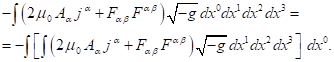
We will use this rule on the left-hand side of
(5), and then integrate (5) with respect to the invariant four-volume,
replacing ![]() by
by ![]() :
:
![]() . (6)
. (6)
The tensor ![]() in (6) is the electromagnetic field tensor
with mixed indices. We will now use the divergence theorem and transform the
left-hand side in (6):
in (6) is the electromagnetic field tensor
with mixed indices. We will now use the divergence theorem and transform the
left-hand side in (6):
![]() , (7)
, (7)
where ![]() is the orthonormal differential
is the orthonormal differential ![]() of the hypersurface surrounding the physical
system in the four-dimensional space,
of the hypersurface surrounding the physical
system in the four-dimensional space, ![]() is the four-dimensional normal vector
perpendicular to the hypersurface and directed outward.
is the four-dimensional normal vector
perpendicular to the hypersurface and directed outward.
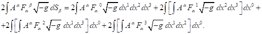
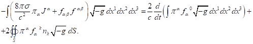
In (6) and (7) we may not perform integration
with respect to the time coordinate ![]() and may consider the physical system at a
fixed arbitrary time point. To this end, we will rewrite the right-hand sides
of (6) and (7):
and may consider the physical system at a
fixed arbitrary time point. To this end, we will rewrite the right-hand sides
of (6) and (7):
 (8)
(8)
 (9)
(9)
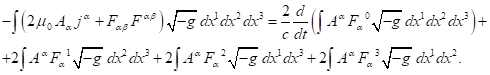
The right-hand sides in (8) and (9) are equal to
each other as a consequence of (6). Now we will differentiate them with respect
to the variable ![]() ,
where
,
where ![]() is the speed of light,
is the speed of light, ![]() is the coordinate time, and then
equate the results to each other:
is the coordinate time, and then
equate the results to each other:
The last three integrals on the right-hand side
can be combined into one surface integral taken over the closed two-dimensional
surface ![]() ,
inside which the entire system with all the particles and fields must be
located. All this gives the following:
,
inside which the entire system with all the particles and fields must be
located. All this gives the following:
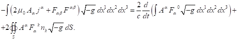 (10)
(10)
In (10) the three-dimensional unit vector ![]() ,
where
,
where ![]() , is the
normal vector to the surface
, is the
normal vector to the surface ![]() directed outward.
directed outward.
In many practical cases, the right-hand side of
(10) vanishes. In particular, the electromagnetic field of the system is
present both inside and outside the system up to infinity. Then the last
integral on the right-hand side of (10) is the surface integral over a surface
of infinitely large radius. But for a closed system, in which there are only
the proper fields of the system’s particles, both the four-potential ![]() and the electromagnetic field tensor
and the electromagnetic field tensor ![]() vanish at infinity due to the gauge of the
potentials, field strength and magnetic field. Consequently, for a closed
system this integral in (10) is equal to zero. If the derivative with respect
to time inside of the first integral on the right-hand side of (10) is also
equal to zero, then the following relation would hold for the left-hand side:
vanish at infinity due to the gauge of the
potentials, field strength and magnetic field. Consequently, for a closed
system this integral in (10) is equal to zero. If the derivative with respect
to time inside of the first integral on the right-hand side of (10) is also
equal to zero, then the following relation would hold for the left-hand side:
![]() . (11)
. (11)
The quantities
inside the integral in (11) are often used in various calculations.
For example, the Lagrangian for four vector fields, including the
electromagnetic field, in case of continuous medium has the following form [1]:
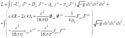 (12)
(12)
where ![]() is a certain coefficient to be determined,
is a certain coefficient to be determined,
![]() is the scalar curvature,
is the scalar curvature,
![]() is the cosmological constant,
is the cosmological constant,
![]() is the four-vector of the mass current,
is the four-vector of the mass current,
![]() is the mass density in the reference frame associated with the particle,
is the mass density in the reference frame associated with the particle,
![]() is the four-velocity of a point particle,
is the four-velocity of a point particle, ![]() is the
four-displacement, and
is the
four-displacement, and ![]() is the interval,
is the interval,
![]() is the four-potential of the acceleration field, where
is the four-potential of the acceleration field, where ![]() and
and ![]() denote the
scalar and vector potentials, respectively,
denote the
scalar and vector potentials, respectively,
![]() is the four-potential of the gravitational field, described through the
scalar potential
is the four-potential of the gravitational field, described through the
scalar potential ![]() and the vector potential
and the vector potential ![]() of this field,
of this field,
![]() is the four-potential of the pressure field, consisting of the scalar potential
is the four-potential of the pressure field, consisting of the scalar potential ![]() and the vector potential
and the vector potential ![]() ,
,
![]() is the gravitational constant,
is the gravitational constant,
![]() is the gravitational tensor,
is the gravitational tensor,
![]() is the
definition of the gravitational tensor with contravariant indices using the
metric tensor
is the
definition of the gravitational tensor with contravariant indices using the
metric tensor ![]() ,
,
![]() is the four-potential of the electromagnetic
field, defined by the scalar potential
is the four-potential of the electromagnetic
field, defined by the scalar potential ![]() and the vector potential
and the vector potential ![]() of this field,
of this field,
![]() is the
four-vector of the charge current,
is the
four-vector of the charge current,
![]() is the charge
density in the reference frame associated with the particle,
is the charge
density in the reference frame associated with the particle,
![]() is the acceleration field
tensor, calculated using the curl of the four-potential of the acceleration field,
is the acceleration field
tensor, calculated using the curl of the four-potential of the acceleration field,
![]() is the acceleration field
coefficient,
is the acceleration field
coefficient,
![]() is the pressure field tensor,
is the pressure field tensor,
![]() is the pressure
field coefficient.
is the pressure
field coefficient.
In (12) the
gravitational field is considered as a vector field in the framework of the
covariant theory of gravitation. If (11) holds true, then in (12) the term ![]() is half as large as the term
is half as large as the term ![]() , and has the opposite sign.
, and has the opposite sign.
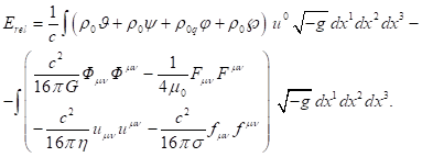
As another example we will give the expression
for the relativistic energy of a physical system of particles and four vector
fields, also in the approximation of continuous medium [1]:
 (13)
(13)
If (11) is satisfied in such a system, then the
integral of the quantity ![]() over the infinite volume in (13) can be
replaced by the integral of the quantity
over the infinite volume in (13) can be
replaced by the integral of the quantity ![]() over the volume occupied by the matter. This
would allow us to significantly simplify the calculation of the system’s
energy.
over the volume occupied by the matter. This
would allow us to significantly simplify the calculation of the system’s
energy.
The classical virial theorem for the kinetic
energy ![]() of the system’s particles and the potential
energy
of the system’s particles and the potential
energy ![]() of these particles is written as follows:
of these particles is written as follows: ![]() . Comparison
of (13) and (11) shows that in some cases a quantitatively opposite relation of
the form
. Comparison
of (13) and (11) shows that in some cases a quantitatively opposite relation of
the form ![]() is satisfied for the electromagnetic field. In
this case
is satisfied for the electromagnetic field. In
this case
![]() ,
,
![]() ,
,
so that ![]() plays the role of the kinetic energy of the
field in the interaction of the four-potential
plays the role of the kinetic energy of the
field in the interaction of the four-potential ![]() with the charge four-current
with the charge four-current ![]() of the particles, and
of the particles, and ![]() characterizes the potential energy of the
field, not that of the particles.
characterizes the potential energy of the
field, not that of the particles.
3. The integral theorem of energy
for other vector fields
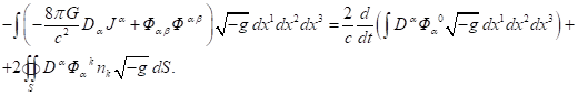
In the covariant theory of gravitation [1] the
description of the gravitational field occurs in the same way as it is done for
the electromagnetic field. This means similarity of the equations of both
fields, and we can immediately write the integral theorem of energy for the
gravitational field, replacing in (10) the notation of the four-current,
four-potential and field tensor, and replacing ![]() by
by ![]() :
:
 (14)
(14)
If the physical system is closed, then in (14)
the last surface integral on the right-hand side would vanish as a consequence
of the field gauge at infinity, where the four-potential ![]() and the gravitational field tensor
and the gravitational field tensor ![]() of the system must be equal to zero.
of the system must be equal to zero.
Similarly, we can proceed with the acceleration
field and with the vector pressure field [2], for which the integral theorem of
the field energy is written as follows:
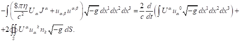 (15)
(15)
 (16)
(16)
However, the acceleration field and the pressure
field differ substantially from the electromagnetic and gravitational fields,
because they act only within the limits of matter. Therefore, in (15) and (16)
the surface integrals on the right-hand side should be taken over the outer
surface of the volume occupied by the system’s matter.
4. Application of the integral
theorem of energy in the relativistic uniform system
A relativistic uniform system is a suitable
object for testing many physical laws. Thus in [3] we studied the virial
theorem and found out the difference from the classical approach due to taking
into account the relativistic corrections. In [4] we applied the formulas,
derived for a relativistic uniform system, to planets and stars and found good
agreement with the results of other authors. Besides we assumed that the matter
is in random motion, the matter particles do not have proper rotation and there
are no directed fluxes of matter. As a result, in this system under
consideration both the global vector potentials of all the fields and the
global solenoidal field vectors vanish. For example, for the electromagnetic
field this means that both the global vector potential ![]() and the magnetic field
and the magnetic field ![]() are equal to zero. A more thorough analysis
shows that each charged moving typical particle has its own small vector
potential
are equal to zero. A more thorough analysis
shows that each charged moving typical particle has its own small vector
potential ![]() , which is
proportional to the instantaneous velocity
, which is
proportional to the instantaneous velocity ![]() of the particle and to the proper electric
scalar potential
of the particle and to the proper electric
scalar potential ![]() of the particle, as well as its own magnetic
field
of the particle, as well as its own magnetic
field ![]() . The
contribution from
. The
contribution from ![]() and
and ![]() in the subsequent calculations is small due to
the small value of the charge of each particle, therefore it can be neglected
in the first approximation. The same also applies to the corresponding values
for the gravitational field.
in the subsequent calculations is small due to
the small value of the charge of each particle, therefore it can be neglected
in the first approximation. The same also applies to the corresponding values
for the gravitational field.
Let us now consider how the integral theorem of
energy is satisfied for the electromagnetic field in the case of a relativistic
uniform system. We will assume that the system is closed, has a spherical shape
and is held in equilibrium under the action of the forces from gravitational
attraction and the repulsion forces from the electromagnetic field and the
pressure field. The acceleration field also contributes to the equilibrium of
forces, since at random motion inside the sphere the particles experience a
centripetal force from the particles’ velocity component, which is tangential
with respect to the sphere’s radius. We will use the approximation of
continuous medium, so the intervals between typical particles are minimal and
we can assume that the sphere’s volume consists of the volumes of particles.
In order to simplify the subsequent calculations we will consider the situation within the
framework of the special theory of relativity, in which ![]() .
.
For a closed system the surface integral in (10)
vanishes and for the electromagnetic field we have the following:
![]() .
(17)
.
(17)
Since ![]() , and in the first approximation we
consider that in the system under consideration
, and in the first approximation we
consider that in the system under consideration ![]() , then in
order to calculate the four-potential we also need to know the distribution of
the global electric potential
, then in
order to calculate the four-potential we also need to know the distribution of
the global electric potential ![]() in the system. As was found in [5], the
electric potential inside the sphere depends on the sinusoidal functions:
in the system. As was found in [5], the
electric potential inside the sphere depends on the sinusoidal functions:
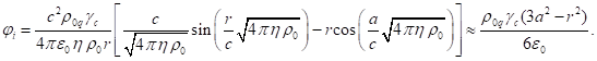
(18)
In (18) ![]() is the electric constant,
is the electric constant, ![]() is the Lorentz factor of the particles at the
center of the sphere,
is the Lorentz factor of the particles at the
center of the sphere, ![]() is the radius of the sphere. For the charge
four-current we have:
is the radius of the sphere. For the charge
four-current we have: ![]() , while the
four-velocity is
, while the
four-velocity is ![]() , where
, where ![]() is the Lorentz factor for the particles,
is the Lorentz factor for the particles, ![]() is the particles’ velocity. The dependence of
is the particles’ velocity. The dependence of ![]() on the current radius
on the current radius ![]() is as follows [6]:
is as follows [6]:
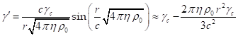 . (19)
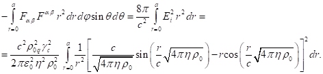
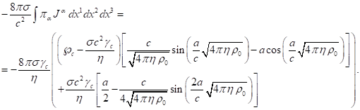
With this in mind, for the scalar product of the
four-vectors we find: ![]() .
Now, using (18) and (19), we can calculate the first term on the left-hand side
of (17):
.
Now, using (18) and (19), we can calculate the first term on the left-hand side
of (17):

In the spherical coordinates ![]() , and
this integral will equal:
, and
this integral will equal:
(20)
In (20), the charge ![]() is the product of the particles’ invariant
charge density
is the product of the particles’ invariant
charge density ![]() by the sphere’s volume, and likewise, the mass
by the sphere’s volume, and likewise, the mass
![]() is the product of the particles’ invariant
mass density
is the product of the particles’ invariant
mass density ![]() by the sphere’s volume. The quantities
by the sphere’s volume. The quantities ![]() and
and ![]() have a technical character and they are not
equal to the sphere’s total charge
have a technical character and they are not
equal to the sphere’s total charge ![]() and the gravitational mass
and the gravitational mass ![]() , respectively.
In particular, according to [5],
, respectively.
In particular, according to [5],
(21)
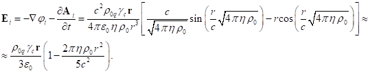
In view of (18) and the equality of the vector
potential to zero, that is, ![]() , the electric field strength inside the sphere
can be determined by the formula:
, the electric field strength inside the sphere
can be determined by the formula:
(22)
Similarly, the electric field strength outside
the sphere is equal to:
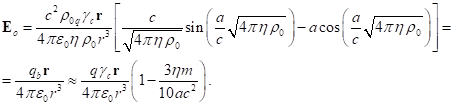 (23)
(23)
In the general case, the electromagnetic field
tensor ![]() contains the components of the electric field
strength vector
contains the components of the electric field
strength vector ![]() and the magnetic field vector
and the magnetic field vector ![]() . In the
system under consideration, on the average
. In the
system under consideration, on the average ![]() , while in
the Cartesian space coordinates
, while in
the Cartesian space coordinates ![]() ,
, ![]() ,
, ![]() , and the
remaining components of the tensors
, and the
remaining components of the tensors ![]() and
and ![]() are assumed to be equal to zero. Therefore, in
this case
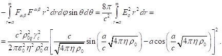
are assumed to be equal to zero. Therefore, in
this case ![]() . The
integral over the volume inside the sphere taken for the second term on the
left-hand side of (17), in view of (22), in the spherical coordinates is equal
to:
. The
integral over the volume inside the sphere taken for the second term on the
left-hand side of (17), in view of (22), in the spherical coordinates is equal
to:
This integral must be taken by parts, placing ![]() under the differential sign in the form
under the differential sign in the form ![]() . This gives
the following:
. This gives
the following:
 (24)
(24)
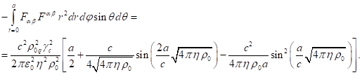
Let us now calculate the integral over the volume
outside the sphere taken for the second term on the left-hand side of (17), in
view of (23), in the spherical coordinates:
 (25)
(25)
The sum of (24) and (25) gives the integral over
the entire space:
(26)
If we take into account the identity ![]() and substitute (20) and (26) into (17), then
we can see that the left-hand side of (17) becomes equal to zero. Therefore, in
the given physical system the right-hand side of (17) must also be equal to
zero:
and substitute (20) and (26) into (17), then
we can see that the left-hand side of (17) becomes equal to zero. Therefore, in
the given physical system the right-hand side of (17) must also be equal to
zero:
![]() . (27)
. (27)
And this is true, since the space components of
the four-potential ![]() are assumed to be equal to zero, that is,
are assumed to be equal to zero, that is, ![]() . At the
same time, the time component of the electromagnetic field tensor is equal to
zero due to antisymmetry of the tensor,
. At the
same time, the time component of the electromagnetic field tensor is equal to
zero due to antisymmetry of the tensor, ![]() .
Consequently, the product
.
Consequently, the product ![]() , and
equation (27) is satisfied.
, and
equation (27) is satisfied.
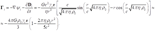
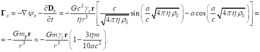
For the gravitational field the situation is
completely analogous to that of the electromagnetic field. For a closed system,
within the framework of the special theory of relativity, in (14) the surface
integral vanishes and we have the following:
![]() . (28)
. (28)
Since in the relativistic uniform system the
global vector potential of the gravitational field is equal to zero, ![]() ,
both the product
,
both the product ![]() and the right-hand side of (28) are equal to
zero. As for the left-hand side of (28), in order to calculate it we need the
global scalar gravitational potential
and the right-hand side of (28) are equal to
zero. As for the left-hand side of (28), in order to calculate it we need the
global scalar gravitational potential ![]() inside the sphere and the gravitational field
strengths inside and outside the sphere [5]:
inside the sphere and the gravitational field
strengths inside and outside the sphere [5]:
 .
.
(29)
(30)
(31)
We obtain the product ![]() as follows:
as follows: ![]() . Then
taking into account (19) and (29), for the first term on the left-hand side of
(28) we find:
. Then
taking into account (19) and (29), for the first term on the left-hand side of
(28) we find:
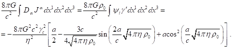 (32)
(32)
For the second term on the left-hand side of
(28), in view of (30) and (31) we have the following:
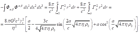 (33)
(33)
The sum of (32) and (33) vanishes according to
(28), where the right-hand side is equal to zero.
5. The
acceleration field
Let us begin with clarification of
what should be meant by the four-potential of the acceleration field of a certain
physical system in the general case. According to [2], the four-potential of
any vector field, the vector potential of which is equal to zero in its proper
reference frame, that is, in the center-of-momentum frame, in case of
rectilinear motion in the laboratory reference frame can be defined by the
following formula:
![]() , (34)
, (34)
where ![]() for the electromagnetic field and
for the electromagnetic field and ![]() for the remaining fields;
for the remaining fields; ![]() is the invariant energy density of interaction, which is the product of the four-potential of the field by the
corresponding 4-current;
is the invariant energy density of interaction, which is the product of the four-potential of the field by the
corresponding 4-current; ![]() is the four-velocity with a covariant index
that defines the motion of the center of momentum of the physical system in the
laboratory reference frame.
is the four-velocity with a covariant index
that defines the motion of the center of momentum of the physical system in the
laboratory reference frame.
In the proper reference frame ![]() , and the vector potential as the
space component
, and the vector potential as the
space component ![]() vanishes according to (34). However, some
physical systems, even if their center of momentum is fixed, have not only a
scalar potential but also a vector field potential within the system.
Therefore, the more general expression for the four-potential of the field in
the laboratory reference frame is as follows:
vanishes according to (34). However, some
physical systems, even if their center of momentum is fixed, have not only a
scalar potential but also a vector field potential within the system.
Therefore, the more general expression for the four-potential of the field in
the laboratory reference frame is as follows:
![]() , (35)
, (35)
where ![]() is a matrix connecting the coordinates and
time of two reference frames, one of which is the laboratory reference frame
and the other moves together with the center of momentum of the physical system
under consideration, so that it has the four-potential
is a matrix connecting the coordinates and
time of two reference frames, one of which is the laboratory reference frame
and the other moves together with the center of momentum of the physical system
under consideration, so that it has the four-potential ![]() of the field in it. In the special case of the
system’s motion at the constant velocity
of the field in it. In the special case of the
system’s motion at the constant velocity ![]() represents the Lorentz transformation matrix [7].
represents the Lorentz transformation matrix [7].
As a typical example we will consider
a neutron star consisting mainly of neutrons and to some extent of protons and
electrons. Both the star itself and the nucleons have fast rotation and strong
magnetic fields. Despite the absence of charge, each neutron has a complex
internal electromagnetic structure and a magnetic moment. Suppose that it is
required to model a star as a relativistic uniform system and to specify the
four-potential of the field of an arbitrary moving nucleon as a typical
particle. To do this, we must use formula (35), since in (34) it is assumed
that there is no vector potential in the nucleon’s center-of-momentum frame.
Really, a nucleon may not move in space, but due to proper rotation and complex
internal structure in the nucleon there are nonzero vector potentials of almost
all the fields.
In order to simplify the
calculations, we will further assume that the physical system under
consideration does not have general rotation, the system’s typical particles
move randomly and have neither proper rotation, nor proper vector potentials in
the center-of-momentum frames of the particles. In this case, we can use a
simpler formula (34) instead of (35).
In a fixed sphere, the energy density
in the volume of each particle is ![]() , and for the acceleration field in
case of rectilinear motion of the sphere in the laboratory reference frame,
according to (34), the four-potential will equal
, and for the acceleration field in
case of rectilinear motion of the sphere in the laboratory reference frame,
according to (34), the four-potential will equal ![]() . This means that if for an observer
inside the sphere with particles within the relativistic uniform model the
quantity
. This means that if for an observer
inside the sphere with particles within the relativistic uniform model the
quantity ![]() is an invariantly determined Lorentz factor as
a certain function of coordinates and time, then for an observer in the
laboratory reference frame, in which the sphere’s center has the four-velocity
is an invariantly determined Lorentz factor as
a certain function of coordinates and time, then for an observer in the
laboratory reference frame, in which the sphere’s center has the four-velocity ![]() , the four-potential of the
acceleration field for each point inside
the moving sphere will equal
, the four-potential of the
acceleration field for each point inside
the moving sphere will equal ![]() .
.
In the ideal case, when the system of
particles is an absolutely solid body and the particles inside the system are
motionless, it should be ![]() , and then the four-potential of the
acceleration field would coincide with the four-velocity of the system’s center
of momentum,
, and then the four-potential of the
acceleration field would coincide with the four-velocity of the system’s center
of momentum, ![]() . A material point is a tiny
physical system, and if we do not delve deeply into the structure of the
internal motion of its matter and consider this point as a solid body, then the
four-potential of the acceleration field of such a point would be equal to the
four-velocity of its rectilinear motion.
. A material point is a tiny
physical system, and if we do not delve deeply into the structure of the
internal motion of its matter and consider this point as a solid body, then the
four-potential of the acceleration field of such a point would be equal to the
four-velocity of its rectilinear motion.
By definition, the four-potential of
the acceleration field is a four-vector ![]() , where
, where ![]() and
and ![]() denote the scalar and vector potentials,
respectively. In view
of (34) and the relation
denote the scalar and vector potentials,
respectively. In view
of (34) and the relation ![]() , it turns out that in the
relativistic uniform system under consideration in the form of a fixed sphere
the scalar potential will be
, it turns out that in the
relativistic uniform system under consideration in the form of a fixed sphere
the scalar potential will be ![]() . As for the global vector potential of the
acceleration field
. As for the global vector potential of the
acceleration field ![]() , it is equal to zero due to the
randomness of motion of the matter particles. On the other hand, inside each
typical particle there is always a small vector potential
, it is equal to zero due to the
randomness of motion of the matter particles. On the other hand, inside each
typical particle there is always a small vector potential ![]() of the acceleration field, which is
proportional to the instantaneous velocity
of the acceleration field, which is
proportional to the instantaneous velocity ![]() of the particle. This changes to some extent
the form of the effectively acting four-potential of the acceleration field
inside the sphere.
of the particle. This changes to some extent
the form of the effectively acting four-potential of the acceleration field
inside the sphere.
Let an arbitrary typical particle
move inside the sphere, and its four-velocity within the framework of the
special theory of relativity ![]() , where
, where ![]() is the velocity of the particle,
is the velocity of the particle, ![]() is the Lorentz factor of the particle. This
particle, in turn, can be considered as a relativistic uniform system, in which
subparticles with the Lorentz factor
is the Lorentz factor of the particle. This
particle, in turn, can be considered as a relativistic uniform system, in which
subparticles with the Lorentz factor ![]() move randomly relative to the particle’s
center of momentum. Then, according to (34), the four-potential of the
acceleration field for this moving particle will be written as
move randomly relative to the particle’s
center of momentum. Then, according to (34), the four-potential of the
acceleration field for this moving particle will be written as ![]() . Comparison with the expression
. Comparison with the expression 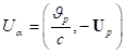 allows us to determine the acceleration field
potentials inside each moving particle of the sphere:
allows us to determine the acceleration field
potentials inside each moving particle of the sphere: ![]() ,
,
![]() . In this case it turns out that
. In this case it turns out that ![]() , that is, the motion of
subparticles inside the particle with the Lorentz factor
, that is, the motion of
subparticles inside the particle with the Lorentz factor ![]() increases the scalar potential of the moving
particle up to the value
increases the scalar potential of the moving
particle up to the value ![]() .
.
Due to the
smallness of the local vector potential ![]() , we will not use it in our calculations. As a result, for the
four-potential of the acceleration field inside the sphere we can write the
following:
, we will not use it in our calculations. As a result, for the
four-potential of the acceleration field inside the sphere we can write the
following:
![]() . (36)
. (36)
This means that we do not take into
account the internal motion of subparticles in individual particles, assuming
that ![]() , so that the scalar potential of
the particles will be equal to
, so that the scalar potential of
the particles will be equal to ![]() and will coincide with the acceleration field
potential inside the fixed sphere.
and will coincide with the acceleration field
potential inside the fixed sphere.
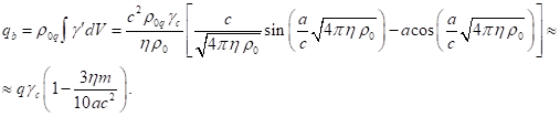
5.1 Calculation for the acceleration field
Given that the mass four-current is ![]() , and the effective four-potential
of the acceleration field inside the sphere is determined in (36), we find that
, and the effective four-potential
of the acceleration field inside the sphere is determined in (36), we find that
![]() .
.
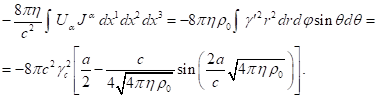
Now we can write the first part of
the integral on the left-hand side of (15) and in view of (19) we can perform integration
in the spherical coordinates:
Since the acceleration tensor is
defined by the expression ![]() , then in view of (36) the tensor
invariant has the following form:
, then in view of (36) the tensor
invariant has the following form: ![]() .
.
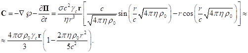
The acceleration field strength
inside the sphere is calculated in terms of the scalar and vector potentials [2],
and since ![]() ,
, ![]() , according to (36), then in view of (19) we obtain:
, according to (36), then in view of (19) we obtain:
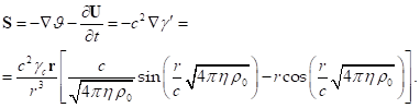 (38)
(38)
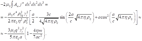
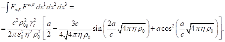
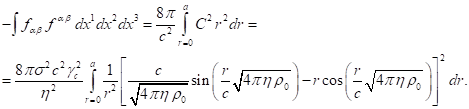
Using (38) we will calculate the
following integral over the sphere’s volume:
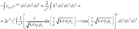
This integral
can be calculated similarly to (24) in the spherical coordinates:
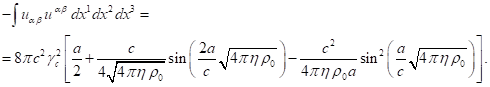 (39)
(39)
Let us now go
over to the right-hand side of (15), for which it is necessary to calculate the
product ![]() inside the sphere. If according to (36) the
four-potential has the components
inside the sphere. If according to (36) the
four-potential has the components ![]() , then the time components of the
acceleration tensor in the Cartesian space coordinates are
, then the time components of the
acceleration tensor in the Cartesian space coordinates are ![]() ,
, ![]() ,
, ![]() ,
, ![]() . Consequently,
. Consequently, ![]() , and the first integral on the right-hand
side of (15) is equal to zero.
, and the first integral on the right-hand
side of (15) is equal to zero.
We
have also to calculate the surface integral on the right-hand side of (15). If
we introduce the vector ![]() , then we see that the surface integral reduces to a doubled flux of
this vector through the spherical surface of the system.
, then we see that the surface integral reduces to a doubled flux of
this vector through the spherical surface of the system.
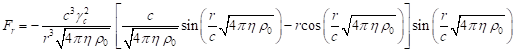
The radial component of the vector ![]() is defined by the expression
is defined by the expression ![]() , where
, where ![]() is a unit vector directed along
the radius. To determine the doubled flux of the vector
is a unit vector directed along
the radius. To determine the doubled flux of the vector ![]() it suffices to multiply the value
it suffices to multiply the value
![]() , calculated at
, calculated at ![]() , by the doubled area of the sphere:
, by the doubled area of the sphere:
![]() . (40)
. (40)
Since
according to (36) the four-potential of the acceleration field inside the
sphere has the components ![]() , and the nonzero components of the
acceleration tensor in the Cartesian space coordinates equal
, and the nonzero components of the
acceleration tensor in the Cartesian space coordinates equal ![]() ,
, ![]() ,
, ![]() , then it should be:
, then it should be:
![]() ,
,
![]() .
.
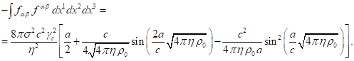
In view of
(19) and (38), we find:
 .
.
At ![]() this expression gives
this expression gives ![]() , and then the surface integral (40)
is calculated as follows:
, and then the surface integral (40)
is calculated as follows:
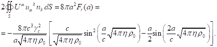
(41)
Substituting (37), (39), and (41) into (15), we
can see that the theorem of energy for the acceleration field is exactly
satisfied.
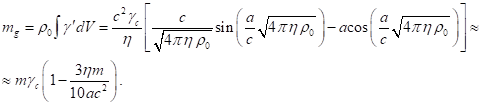
6. The pressure field
In
the physical system under consideration the vector potential ![]() is assumed to be equal to zero, and then the
four-potential of the pressure field inside the sphere in the approximation of
the special theory of relativity will be written as follows:
is assumed to be equal to zero, and then the
four-potential of the pressure field inside the sphere in the approximation of
the special theory of relativity will be written as follows:
![]() . (42)
. (42)
The
scalar potential of the pressure field was calculated in [6]:
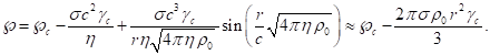 (43)
(43)
The
mass four-current has the following form: ![]() . With this in mind
. With this in mind ![]() , and we can write the first
integral on the left-hand side of (16):
, and we can write the first
integral on the left-hand side of (16):
![]() .
.
Substituting
here (43) and ![]() from (19), we find:
from (19), we find:
(44)
Since
we assumed that in the system under consideration the vector potential of the
pressure field is absent, then the solenoidal vector ![]() of the pressure field, calculated as the curl
of the vector potential [2], will also be equal to zero. In this case, the
pressure field tensor
of the pressure field, calculated as the curl
of the vector potential [2], will also be equal to zero. In this case, the
pressure field tensor ![]() will depend only on the field strength
will depend only on the field strength ![]() , so that the tensor invariant will
equal
, so that the tensor invariant will
equal ![]() . The pressure field strength is
determined by the formula:
. The pressure field strength is
determined by the formula:
 (45)
(45)
Now
we can write the second integral on the left-hand side of (16) in the spherical
coordinates:
This integral
is calculated in the same way as (24):
 (46)
(46)
On
the right-hand side of (16) there is a product ![]() , and the pressure field tensor
components are the following:
, and the pressure field tensor
components are the following: ![]() ,
, ![]() ,
, ![]() ,
, ![]() . If we take into account the
components of the four-potential
. If we take into account the
components of the four-potential ![]() according to (42), then we can see that
according to (42), then we can see that ![]() .
.
Now
we will turn to the product ![]() on the right-hand side of (16), where
on the right-hand side of (16), where ![]() . Since the four-potential
. Since the four-potential ![]() contains only the time component with the
index
contains only the time component with the
index ![]() , we will write out all the nonzero
components of
, we will write out all the nonzero
components of ![]() :
: ![]() ,
, ![]() ,
, ![]() . Consequently, the product
. Consequently, the product ![]() is a radial vector directed oppositely to the
pressure field strength vector
is a radial vector directed oppositely to the
pressure field strength vector ![]() . The fact that
. The fact that ![]() is a radial vector allows us immediately to
find the surface integral on the right-hand side of (16). To calculate this
integral, we need to assume
is a radial vector allows us immediately to
find the surface integral on the right-hand side of (16). To calculate this
integral, we need to assume ![]() in the field strength
in the field strength ![]() (45) and in the scalar potential
(45) and in the scalar potential ![]() (43), which are part of
(43), which are part of ![]() , and then to multiply
, and then to multiply ![]() by the normal vector
by the normal vector ![]() , and multiply the obtained result
by the area of the sphere’s surface:
, and multiply the obtained result
by the area of the sphere’s surface:
 (47)
(47)
Substituting
the expressions from (44), (46) and (47) into (16), we find that the theorem of
energy for the pressure field is satisfied, since all the terms in (16)
completely cancel out with each other.
7. Conclusion
By
the example of the electromagnetic field we derived the integral theorem of the
field energy in relation (10). In addition, we introduced the concepts of the
kinetic energy ![]() and the potential energy
and the potential energy ![]() of the electromagnetic field:
of the electromagnetic field:
![]() ,
, ![]() . (48)
. (48)
In
(48), the energy ![]() is related to the energy of interaction of the
field and particles and is calculated in terms of the product of the
four-potential
is related to the energy of interaction of the
field and particles and is calculated in terms of the product of the
four-potential ![]() of the field and the charge four-current
of the field and the charge four-current ![]() of the particles, and the energy
of the particles, and the energy ![]() is expressed in terms of the volume integral
of the tensor invariant
is expressed in terms of the volume integral
of the tensor invariant ![]() of the electromagnetic field. From (10) and
(48) we obtain the following relation:
of the electromagnetic field. From (10) and
(48) we obtain the following relation:
![]() . (49)
. (49)
For
a closed system, the surface integral on the right-hand side of (49) vanishes
due to the gauge of the four-potential ![]() and the electromagnetic field tensor
and the electromagnetic field tensor ![]() at infinity. In the relativistic uniform system the product
at infinity. In the relativistic uniform system the product ![]() also vanishes, and then (49) reduces to a
simple relation
also vanishes, and then (49) reduces to a
simple relation ![]() . This relation for the field
resembles the classical virial theorem for particles of the form
. This relation for the field
resembles the classical virial theorem for particles of the form ![]() , where
, where ![]() is kinetic energy, and
is kinetic energy, and ![]() is the potential energy of the particles. The
relation
is the potential energy of the particles. The
relation ![]() is often used in electrostatics, allowing to
determine the electrical energy of the system in two different ways – either
with the charge density and the electric potential, or with the field strength,
which is part of the electromagnetic tensor. However, in the general case there
was no proof of existence of a relationship between the energies (48) in the
presence of electric currents and magnetic fields. Now we see that such a
relationship in (49) is the consequence of the integral theorem of the field energy.
is often used in electrostatics, allowing to
determine the electrical energy of the system in two different ways – either
with the charge density and the electric potential, or with the field strength,
which is part of the electromagnetic tensor. However, in the general case there
was no proof of existence of a relationship between the energies (48) in the
presence of electric currents and magnetic fields. Now we see that such a
relationship in (49) is the consequence of the integral theorem of the field energy.
In
(14) we presented the integral theorem of energy for the vector gravitational
field in the framework of the covariant theory of gravitation, and in (15) and
(16) – the integral theorem of energy for the acceleration field and the
pressure field, respectively. By analogy with (48), for these fields we can
also introduce the concepts of the kinetic energy and the potential energy of
the field. In particular, in [8] for closed static uniform systems it was found
that a relation of the form ![]() holds in them for the gravitational field.
holds in them for the gravitational field.
For
all the four vector fields in Sections 4, 5 and 6 we showed by direct
calculation of all the terms in the formulation of the integral theorem of
energy how exactly this theorem is satisfied in the case of a relativistic
uniform system. These calculations prove that the integral theorem of the field
energy is exactly satisfied, confirming the validity of the theorem.
References
1. Fedosin
S.G. About the cosmological constant, acceleration
field, pressure field and energy. Jordan
Journal of Physics. Vol. 9, No. 1,
pp. 1-30 (2016).
doi:10.5281/zenodo.889304.
2. Fedosin
S.G. The procedure of
finding the stress-energy tensor and vector field equations of any form. Advanced Studies in Theoretical
Physics. Vol. 8, pp. 771-779 (2014). doi: 10.12988/astp.2014.47101.
3. Fedosin
S.G. The virial theorem and the kinetic energy of particles
of a macroscopic system in the general field concept. Continuum Mechanics and Thermodynamics, Vol. 29, Issue 2,
pp. 361-371 (2016). doi:10.1007/s00161-016-0536-8.
4. Fedosin
S.G. Estimation of the physical parameters of
planets and stars in the gravitational equilibrium model. Canadian Journal of Physics, Vol. 94, No. 4, pp. 370-379
(2016). doi:10.1139/cjp-2015-0593.
5. Fedosin
S.G. Relativistic Energy and Mass in the Weak Field
Limit. Jordan
Journal of Physics. Vol. 8, No. 1,
pp. 1-16 (2015).
doi:10.5281/zenodo.889210.
6. Fedosin
S.G. The Integral Energy-Momentum 4-Vector and Analysis
of 4/3 Problem Based on the Pressure Field and Acceleration Field. American Journal of Modern Physics, Vol. 3, No. 4, pp. 152-167 (2014). doi:10.11648/j.ajmp.20140304.12.
7. Dennery P. and Krzywicki A. Mathematics for Physicists. Courier Corporation.
p. 138 (2012). ISBN 978-0-486-15712-2.
8. Fedosin
S.G. The Gravitational Field in the Relativistic Uniform Model within the
Framework of the Covariant Theory of Gravitation. International Letters of
Chemistry, Physics and Astronomy, Vol. 78, pp. 39-50 (2018). doi:10.18052/www.scipress.com/ILCPA.78.39.
Source: http://sergf.ru/tfen.htm