As a rule,
the exponents’ values in (6) are small, because  value is small.
In this case, the exponents can be expanded in the small parameter by the rule:
value is small.
In this case, the exponents can be expanded in the small parameter by the rule:  . With this in mind, we obtain:
 .
.
In this
expression, we will take into account that the density of the large ball is
given by the formula:  , and will use (3):
 .
.
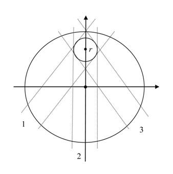
We arrive at
the fact that the force  acts on the small ball in Fig.1, and
this force is directed toward the center of the large ball. By definition, the gravitational
field strength is the ratio of the force, acting on the test body, to the mass
of the test body. Then the vector of the gravitational field strength inside
the large ball will be:
acts on the small ball in Fig.1, and
this force is directed toward the center of the large ball. By definition, the gravitational
field strength is the ratio of the force, acting on the test body, to the mass
of the test body. Then the vector of the gravitational field strength inside
the large ball will be:
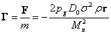 . (7)
. (7)
The minus
sign in (7) is associated with the fact that the force is directed opposite to
the radius vector  .
.
In
Lorentz-invariant theory of gravitation [8], the vector of the gravitational
field strength inside a uniform ball is determined by the formula:
 .
(8)
.
(8)
From
comparison of (7) and (8) we find the expression of the gravitational constant in
terms of the parameters of the graviton field in the approximation of cubic
distribution of graviton fluxes:
 . (9)
. (9)
The
gravitational constant in (9) depends on the cross-section of gravitons’ interaction with the nucleons
of the matter, on the average momentum of one graviton  , on the fluence rate of gravitons
  and on the
nucleon mass
and on the
nucleon mass  . We can repeat the calculations for the case when
instead of nucleons characteristic particles of matter are quarks. Then, in (9) instead of the mass will appear some averaged quark
mass, and the cross-section changes its value, since the
cross-section depends on the kind of interacting particles.
. We can repeat the calculations for the case when
instead of nucleons characteristic particles of matter are quarks. Then, in (9) instead of the mass will appear some averaged quark
mass, and the cross-section changes its value, since the
cross-section depends on the kind of interacting particles.
3. THE GRAVITATIONAL FIELD STRENGTH
OUTSIDE THE UNIFORM BALL
Fig. 1 shows
that the formulas (7) and (9) in cubic distribution were obtained without
taking into account the action of graviton fluxes moving along the inclined
paths of type 1 and 3. The contribution of these fluxes inside the ball is
fixed and depends only on the size of the ball. Therefore, if we add the
contribution of these fluxes, the meaning of formulas (7) and (9) would not
change significantly, except for the appearance of some numerical factors of
the order of unity.
The
situation changes significantly when the test body in the form of a small ball
is outside the large massive ball. In this case, cubic distribution of graviton
fluxes in space becomes too rough for describing these fluxes. After all, in
reality graviton fluxes are directed not only in six mutually perpendicular
directions, but also in any possible directions. So let us move to the
spherical distribution, which is more accurate over long distances, for the
flux of the following form:
 . (10)
In contrast to
(1), for the fluence rate (10) the graviton detector is some spherical surface,
inside of which a number of gravitons  falls from a solid angle
  per time
  . In this case, the origin of this solid angle is at
the center of the said spherical surface and it rests on the surface element area
. In this case, the origin of this solid angle is at
the center of the said spherical surface and it rests on the surface element area  , since it is considered that gravitons fall
perpendicularly onto the detector’s surface. In fact, part of the gravitons
will fall on at the angles,
which differ from the right angle, so that (10) is another approximation to
reality.
, since it is considered that gravitons fall
perpendicularly onto the detector’s surface. In fact, part of the gravitons
will fall on at the angles,
which differ from the right angle, so that (10) is another approximation to
reality.
Further
arguments with some variations repeat the conclusions made from [5] and [7].
Fig. 2 shows two masses, the interaction of which can be estimated using the
fluence rate (10) for spherical distribution.
Similarly to (2), we can assume that exponential decrease in the number of gravitons occurs in the matter as the graviton fluxes travel along the path  in the matter:
 . (11)
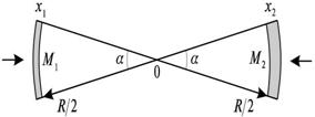
Fig. 2. Masses  and
and  in the form
of ball segments with different thickness and matter density, located at the
distance
in the form
of ball segments with different thickness and matter density, located at the
distance  from each
other
from each
other
For the
masses of ball segments which are attracted to each other we can write:
 ,
,  ,
,  . (12)
The detector
is located at point 0 in the middle between the two segments. For it, each
segment is seen at the same solid angle  at the distance
  , while the transverse areas of the segments are the
same and equal
, while the transverse areas of the segments are the
same and equal  . It means that before we apply further arguments for
the two large bodies, we should cut these bodies into segments and then
calculate the total gravitational force between all the possible pairs of
segments by means of vector summation of particular forces.
. It means that before we apply further arguments for
the two large bodies, we should cut these bodies into segments and then
calculate the total gravitational force between all the possible pairs of
segments by means of vector summation of particular forces.
Decrease of
the graviton flux on the left side after passing the first segment according to
(11) depends on the thickness of this segment and on the concentration of
nucleons:
 .
.
After that
the graviton flux passes through the second segment with further decrease of
the flux:
 .
.
The force
acting on the second segment from the left side with regard to (10) will equal:
 .
.
Decrease of the graviton flux, passing through the second segment from the right side, and the force from this side are, respectively:
 ,
,  .
.
We find the
force of attraction of the second segment to the first one:
 . (13)
This force
is symmetric with respect to changing the segments’ places, so that the first
segment is attracted to the second with the same force.
The
exponents’ values in (13) are small for all space objects, except for the
neutron stars where it is not so. Expanding the exponents in the linear
approximation by the rule , taking into account (12), we obtain for the force
the following:
 .
.
According to
the Newton's law, the formula for the magnitude of the gravitational force
between two bodies is as follows:
 .
.
Comparing
the values of the forces, we arrive at the expression for the gravitational
constant in terms of the graviton field parameters in case of idealized
spherical distribution of graviton fluxes:
 .
(14)
.
(14)
From the expression
for the force we determine the gravitational field strength of one mass at the
location of the second mass:
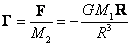 . (15)
4. THE GRAVITON
FIELD PARAMETERS
We will estimate
the energy density for cubic distribution of graviton fluxes in space. Suppose
there is a cube with an edge  , into which gravitons fly from six sides perpendicularly
to the faces of the cube. The speed of gravitons is assumed to be equal to the
speed of light, so that in the time
, into which gravitons fly from six sides perpendicularly
to the faces of the cube. The speed of gravitons is assumed to be equal to the
speed of light, so that in the time  the cube will
be completely filled. In view of distribution (1) the number of gravitons in
the cube will be:
the cube will
be completely filled. In view of distribution (1) the number of gravitons in
the cube will be:  . If the energy of one graviton is
  , then with the
help of (9) for the energy density of the graviton field we find:
, then with the
help of (9) for the energy density of the graviton field we find:
 . (16)
Now we will
use the spherical distribution (10) to estimate the energy density of the
graviton field. An empty sphere with radius  can be filled
with gravitons in the time
can be filled
with gravitons in the time  , if the graviton fluxes are directed radially and
correspond to the full solid angle
, if the graviton fluxes are directed radially and
correspond to the full solid angle  . The number of gravitons inside the sphere will equal
  . Multiplying this number by the energy of one
graviton and dividing by the sphere’s volume we can find the energy density. In view of (14) and the condition
. Multiplying this number by the energy of one
graviton and dividing by the sphere’s volume we can find the energy density. In view of (14) and the condition  , we obtain:
 . (17)
The energy
density (17) with spherical distribution is 3/2 times greater than with cubic
distribution (16), which emphasizes that our estimates are approximate due to
the use of two idealized distributions.
In (16) and
(17) the quantity which is not yet determined is the cross-section of
gravitons’ interaction with the matter  . In [9] for the case when gravitons interact with
electrons in atoms, there is an estimate of the cross-section
. In [9] for the case when gravitons interact with
electrons in atoms, there is an estimate of the cross-section
 , where
  is the Planck
length. In [10] there is a relation for the cross-section:
is the Planck
length. In [10] there is a relation for the cross-section: 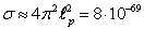 m2, with the conclusion that the
interaction cross-section is only slightly dependent on the type of particles
of matter. All these estimates are based on the fact that the energy of
gravitons is expressed in terms of the Planck constant and the emission
wavelength. But as it will be shown below, from the standpoint of infinite
nesting of matter, gravitons appear primarily not at the level of elementary
particles and atoms, but at the lower levels of matter. And each level of matter
is characterized by its own constant, similar to the Planck constant that
differs from it in value. This fact is taken into account in [11], but since
the energy of gravitons in the form of photons is related to Planck units by
equating the Planck length to the photons’ wavelength, the cross-section of
interaction of these photons with nucleons is overrated and equals
m2, with the conclusion that the
interaction cross-section is only slightly dependent on the type of particles
of matter. All these estimates are based on the fact that the energy of
gravitons is expressed in terms of the Planck constant and the emission
wavelength. But as it will be shown below, from the standpoint of infinite
nesting of matter, gravitons appear primarily not at the level of elementary
particles and atoms, but at the lower levels of matter. And each level of matter
is characterized by its own constant, similar to the Planck constant that
differs from it in value. This fact is taken into account in [11], but since
the energy of gravitons in the form of photons is related to Planck units by
equating the Planck length to the photons’ wavelength, the cross-section of
interaction of these photons with nucleons is overrated and equals  m2.
m2.
In connection
with this, we will take a different approach to determination of cross-section.
We can use as a rough estimate of the relation  for the densest objects with high
concentration of particles
for the densest objects with high
concentration of particles  . According to (2), under this condition, the graviton
flux on the way to the center of the star decreases
. According to (2), under this condition, the graviton
flux on the way to the center of the star decreases  times or more,
where
times or more,
where  is the base of
the natural logarithm.
is the base of
the natural logarithm.
For various
stars of equal mass the product of the concentration and the radius of the star
varies in inverse proportion to the square of the
radius and reaches the maximum with decreasing of the radius. Therefore,
neutron stars as the smallest and densest known objects are most suitable for
estimation of from the condition . If a star were a uniform ball with the radius of 12
km and the mass of 1.35 solar masses, we would have for it  m2.
In [7] we assumed the value of
m2.
In [7] we assumed the value of  m2 for a star with the radius of 15 km, and
we found out that the maximum possible rate of energy generation equaled the rest
energy of the star, that had been released during the time of gravitons’ flight
along the star radius. If we apply the same approach for a star with the radius
of
m2 for a star with the radius of 15 km, and
we found out that the maximum possible rate of energy generation equaled the rest
energy of the star, that had been released during the time of gravitons’ flight
along the star radius. If we apply the same approach for a star with the radius
of  km, we will
obtain:
km, we will
obtain:
 m2 ,
(18)
m2 ,
(18)
where  in case of
uniform density.
in case of
uniform density.
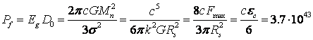
As a
consequence, in [7] we obtained the following value for the limiting force of
attraction between two adjacent massive bodies:
 ,
,
where the case is implied, when the graviton fluxes are completely absorbed by these bodies.
In [5] we considered
the attraction of two neutron stars with minimum distance between them  , while the exponents in the expression for the force
in (13) could not be expanded with respect to the small parameter and were
fully taken into account. This led to the fact that the force of attraction
between the stars decreased in comparison with the Newtonian force
, while the exponents in the expression for the force
in (13) could not be expanded with respect to the small parameter and were
fully taken into account. This led to the fact that the force of attraction
between the stars decreased in comparison with the Newtonian force  and was equal
to the value of the order of
and was equal
to the value of the order of  .
.
Another way
to estimate the cross-section of gravitons’ interaction with the
matter is the following. If we proceed from the similarity of Maxwell equations
for the electromagnetic field and Maxwell-like gravitational equations in the
Lorentz-invariant theory of gravitation [8], [12], then there is a correlation
between the vacuum permittivity  and gravitoelectric constant in the form
  . In addition, the vacuum permeability
  can be related to
gravitomagnetic constant in the form
can be related to
gravitomagnetic constant in the form  , where
  is the speed of gravitation propagation. In case of propagation of
an electromagnetic wave in the vacuum, the wave impedance is determined by the
ratio of the electric field strength amplitude
is the speed of gravitation propagation. In case of propagation of
an electromagnetic wave in the vacuum, the wave impedance is determined by the
ratio of the electric field strength amplitude  to the magnetic
field strength amplitude
to the magnetic
field strength amplitude  :
:
 ,
,
where  is the wave’s magnetic field
induction amplitude.
is the wave’s magnetic field
induction amplitude.
By analogy,
we can determine the gravitational wave impedance of the vacuum [13]. On
condition that the speed of gravitation propagation is equal to the
speed of light we obtain:
 ,
,
where  .
.
The gravitational
wave impedance  must
characterize the propagation of gravitational waves. It is proportional to the ratio
of the amplitude of the gravitational field strength
must
characterize the propagation of gravitational waves. It is proportional to the ratio
of the amplitude of the gravitational field strength  to the
amplitude of the gravitational torsion field
to the
amplitude of the gravitational torsion field  (the latter
quantity in the general theory of relativity is called a gravitomagnetic
field). We will assume that the gravitational quantum has the same
characteristic radius of rotation
(the latter
quantity in the general theory of relativity is called a gravitomagnetic
field). We will assume that the gravitational quantum has the same
characteristic radius of rotation  as in a
circularly polarized photon. For the gravitational Lorentz force we can write the following:
as in a
circularly polarized photon. For the gravitational Lorentz force we can write the following:
 ,
,  ,
,
where the mass  moving at the
velocity
moving at the
velocity  rotates around
the torsion field by a circle with the radius in the same way
as the charge rotates in the magnetic field.
rotates around
the torsion field by a circle with the radius in the same way
as the charge rotates in the magnetic field.
The
amplitude of the gravitational field strength can be related to the amplitude of
the gravitational potential  by a standard
relation:
by a standard
relation:  . If we substitute and into the
expression for , with
. If we substitute and into the
expression for , with  and with the
maximum possible amplitude of the potential
and with the
maximum possible amplitude of the potential  , we will obtain
  .
.
On the other
hand, the mass current in case of circumferential rotation is determined by the
equation:  . Expressing from this
equation and using the relations
. Expressing from this
equation and using the relations  ,
,  and
and  , we obtain the following:
 .
.
Hence it
follows that the gravitational wave impedance for a wave can be treated in the same
way as the gravitational Ohm's law, when the impedance is directly proportional
to the potential difference and inversely proportional to the current. Suppose
now that we have some spherical massive object with the mass  and the radius and the absolute
value of the gravitational potential at its surface reaches the limit value,
which is equal to the square of the speed of light:
and the radius and the absolute
value of the gravitational potential at its surface reaches the limit value,
which is equal to the square of the speed of light:  and
and  . We will estimate the mass current of the graviton
field falling on this object with the help of spherical distribution of
graviton fluxes (10). To do this, we will multiply (10) by the full solid angle
, by the surface area of the sphere
. We will estimate the mass current of the graviton
field falling on this object with the help of spherical distribution of
graviton fluxes (10). To do this, we will multiply (10) by the full solid angle
, by the surface area of the sphere  and by the
energy of one graviton , and then divide by the squared speed of light in
order to move from the energy flux rate to the mass current. Taking into account (17), we find:
and by the
energy of one graviton , and then divide by the squared speed of light in
order to move from the energy flux rate to the mass current. Taking into account (17), we find:
 .
.
Our idea is
that the gravitational wave impedance is the factor of proportionality between
the gravitational potential and the mass current not only in case of the
gravitational wave, but also in case of the mass flux  of the graviton field falling on the
object with the maximum potential. Hence, taking into account the expression for , we obtain the following:
of the graviton field falling on the
object with the maximum potential. Hence, taking into account the expression for , we obtain the following:
 ,
,  ,
,  .
.
In the
latter expression we make substitution , assuming that the object’s mass is the same as
the mass  , that we used
as the mass of the neutron star model, equal to 1.35 Solar masses. This gives:
, that we used
as the mass of the neutron star model, equal to 1.35 Solar masses. This gives:
 m2 ,
m2 ,
which practically coincides with the estimate
in (18). Therefore, we will further use the value of the cross-section of gravitons’
interaction with the matter from (18).
From (16)
and (18) we obtain an estimate of the energy density of the graviton field:
 J/m3. (19)
For comparison,
the density of the absolute value of the gravitational energy in the volume of
the neutron star under consideration is  J/m3,
and the density of the rest energy of the star is
J/m3,
and the density of the rest energy of the star is  J/m3.
J/m3.
The energy
fluence rate as the rate of energy flux of the graviton field in one direction
can be found by multiplying the energy of one graviton by the fluence
rate of gravitons from cubic distribution (1). In view of (9) and (18-19), we find:
 W/m2. (20)
The
cross-section of gravitons’ interaction with matter in (18) is so
small that it can only be compared with the interaction cross-section of
neutrinos with the energy  eV. The
peculiarity of neutrinos is that the cross-section of their interaction with
matter depends mainly on the energy of neutrinos and the concentration of
nucleons, but not on the concentration of electrons.
eV. The
peculiarity of neutrinos is that the cross-section of their interaction with
matter depends mainly on the energy of neutrinos and the concentration of
nucleons, but not on the concentration of electrons.
On the other
hand, if gravitons are the electromagnetic field quanta, then we can equate  to the energy
density of this field, expressed in terms of the emission density constant
to the energy
density of this field, expressed in terms of the emission density constant  and temperature
  . Hence, for the temperature of the graviton field in
the form of photons we find:
. Hence, for the temperature of the graviton field in
the form of photons we find:
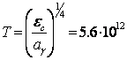 K. (21)
5. INFINITE NESTING OF MATTER
Now we will
correlate the idea of a graviton field with the theory of infinite nesting of
matter [5], [8], [14], according to which in the Universe there are various
similar to each other levels of matter, that differ from each other by their
location on the scale axis. Two major scale levels of matter, such as the
levels of atoms and stars, contain objects with limiting matter density. These
include a neutron and a proton, on the one hand, and their stellar analogues –
a neutron star and a magnetar, on the other hand. Other analogues are
considered to be a muon and a white dwarf, a hydrogen atom and a magnetar with
discon, where a discon is a disc near the neutron star, similar to an electron
disc in the atom. Galaxies correspond to the smallest dust particles, in the
center of which there is solid matter and on the outside there is thick gaseous
shell of the different atoms. The latter analogue becomes thicker over time,
since the stars in the galaxies evolve and turn into neutron stars and white
dwarfs. In this picture magnetars are formed from neutron stars, just as protons are formed from neutrons in beta-decay.
We assume that
black holes do not exist, as they are attributed the property of absorbing
matter and do not letting anything out. But this contradicts the fact that the
graviton field penetrates all bodies, and thereby creates gravitational
phenomena. If a black hole would only absorb the energy of graviton fluxes, it
would acquire in a short time a huge amount of mass-energy and should grow
indefinitely in size, which is not observed.
For objects,
held from decay by gravitation, in [15] we found formulas to estimate the
temperature and pressure at the center of these objects:
 ,
,  , (22)
where  is the
Boltzmann constant,
is the
Boltzmann constant,  is the proton
mass, and the massof the object is contained within the sphere with the
radius .
is the proton
mass, and the massof the object is contained within the sphere with the
radius .
From the relationship
between pressure, concentration of particles and temperature in the center in
the form of  in (22) it
follows that the mass density in the center
in (22) it
follows that the mass density in the center  is about 1.5
times greater than the average mass density
is about 1.5
times greater than the average mass density  of the object:
  .
.
For a neutron
star with the radius of 12 km and the mass of 1.35 solar masses in (22) we
find: the temperature  K; the pressure
  Pa; the mass density
  kg/m3. We must pay attention that the
temperature here is not kinetic, but full generalized temperature. If the
kinetic temperature of ideal gas is determined by the kinetic energy of its
particles, then for a neutron star the generalized temperature is determined by
relation [8]:
kg/m3. We must pay attention that the
temperature here is not kinetic, but full generalized temperature. If the
kinetic temperature of ideal gas is determined by the kinetic energy of its
particles, then for a neutron star the generalized temperature is determined by
relation [8]:  ,
,
where  is the Lagrange
function per one particle. This determination of temperature allows us to take
into account the potential energy of nucleons’ repulsion from each other, which
depends in the gravitational model of the strong interaction on the field of
strong gravitation and on the kinetic energy of nucleons’ rotation [5]. The
motion of nucleons in the star is rather rotational than translational, due to
the high density of matter, and the resulting mutual repulsion of nucleons
opposes the gravitational pressure.
is the Lagrange
function per one particle. This determination of temperature allows us to take
into account the potential energy of nucleons’ repulsion from each other, which
depends in the gravitational model of the strong interaction on the field of
strong gravitation and on the kinetic energy of nucleons’ rotation [5]. The
motion of nucleons in the star is rather rotational than translational, due to
the high density of matter, and the resulting mutual repulsion of nucleons
opposes the gravitational pressure.
We will now
estimate the temperature and pressure in the center of the proton. First we
will introduce the coefficients of similarity as the ratio of the corresponding
quantities. Dividing the mass of the neutron star by the proton mass, we find
the coefficient of similarity in mass:  . Similarly, we calculate the coefficient of
similarity in size as the ratio of the stellar radius to the proton radius:
. Similarly, we calculate the coefficient of
similarity in size as the ratio of the stellar radius to the proton radius:  , here the quantity
  m in the self-consistent model of the proton [16] was
used.
m in the self-consistent model of the proton [16] was
used.
The
coefficient of similarity in speed equals the ratio of the characteristic speeds
of the matter inside the star and the proton, respectively. For the star the
characteristic speed  is calculated
from the energy equality from the standpoint of the general principle of
equivalence of mass and energy, generalized with respect to the absolute value
of the total energy to any space objects:
is calculated
from the energy equality from the standpoint of the general principle of
equivalence of mass and energy, generalized with respect to the absolute value
of the total energy to any space objects:
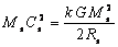 ,
, 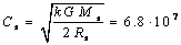 m/s.
m/s.
Similarly, we
find for the proton the equality of the characteristic speed of its matter and
the speed of light:
 m/s, (23)
while  m3·kg-1·s-2 is the
strong gravitational constant, calculated from the equation of electric and gravitational
forces in the hydrogen atom, and according to [16]
m3·kg-1·s-2 is the
strong gravitational constant, calculated from the equation of electric and gravitational
forces in the hydrogen atom, and according to [16]  . Hence, the coefficient of similarity in speed is equal to:
  .
.
The
similarity coefficients allow us to use the relations between similar
quantities of different objects in accordance with the theory of physical dimensions.
For example, the generalized temperature at the center of the proton in view of
(22) must equal:
 , (24)
where  denotes the mass of
particle (praon), while the praon is related to the proton, just as the proton is related to the neutron star [17], and
denotes the mass of
particle (praon), while the praon is related to the proton, just as the proton is related to the neutron star [17], and  is a constant, similar to the Boltzmann constant for the praon level of matter.
From praon
definition we see that  . Besides, according to the theory of dimensions, for
the strong gravitational constant we have
. Besides, according to the theory of dimensions, for
the strong gravitational constant we have  .
.
The
Boltzmann constant has the dimension of
J/K, and if the temperature is not subject to similarity transformation,
then according to the theory of dimensions we will obtain:  . Substituting all this in (24), we arrive at the
equality of generalized temperatures inside the proton and the neutron star:
. Substituting all this in (24), we arrive at the
equality of generalized temperatures inside the proton and the neutron star:
 K. (25)
For the
pressure in the center of the proton similarly to (22) we find:
 Pa.
(26)
Pa.
(26)
We have
found that the pressure in the center of the proton (26) is more than 30 times greater
than the pressure in the center of the neutron star. If we take into account
that 1 Pa = 1 J/m3, then the energy density of the pressure field in
the center of the proton is about three times less than the energy density of
the graviton field (19). The difference of the energy density from the pressure
in the center of the neutron star and the energy density of the graviton field
(19) is up to 90 times.
In addition,
we have the coinciding generalized temperatures in the center of the proton and
the neutron star. According to (25) and (21), the generalized temperature in
the center of these objects is 3 times less than the temperature of the
graviton field, considered as a photon gas. We can explain this by the fact
that gravitons are not fully absorbed by the matter of the neutron star or the
proton, and therefore they cannot heat this matter to their own temperature.
From the
point of view of the theory of similarity of matter levels, we should expect
that at every level of matter the ratio between the energy density of the
graviton field and the energy density of the pressure field in the center of
the densest object is the same. Since the characteristic speed of matter and
the pressure in the center of the proton are higher than the analogous quantities
in the neutron star, then the energy density of the graviton field of strong
gravitation at the atomic level accordingly must be greater. This implies the
dependence of the effective energy density of the graviton field on the level
of matter.
In our
opinion, the main sources of the graviton field at a certain level of matter
are the emissions from the densest objects at the lower levels of matter. For
example, the core of a neutron star is constantly heated under the action of
incident fluxes of gravitons. The degree of heating can be estimated by the
formula (22), which gives the generalized temperature. The kinetic temperature
at the surface of neutron stars is determined from observations and has the
typical value of about 106 K, and the thermal luminosity rarely
exceeds 1026 J/s [18].
Although the
kinetic temperature is less than the generalized temperature, the stellar core
is heated enough to constantly emit neutrino fluxes, escaping from the star and
flowing into the surrounding graviton field. At the time of formation of a
neutron star or during its transformation into a magnetar with reconfiguration
of the magnetic moment, intense neutrino fluxes directed by the magnetic field
(due to the connection between the total magnetic field and the magnetic
moments of nucleons) arise, which will act effectively at a higher level of
matter than the stellar level.
Neutron
stars generate not only neutrino fluxes, but also give rise to cosmic rays, as
it follows from the study of supernova remnants. In [5] and [8] the assumption
is made that magnetars can have a positive electric charge of up to  Cl, where is the elementary electric charge and the
similarity coefficients are used. The proton energy on the
surface of the charged magnetar will reach
Cl, where is the elementary electric charge and the
similarity coefficients are used. The proton energy on the
surface of the charged magnetar will reach  J or
J or  eV. For comparison, the highest recorded values of
cosmic ray energies per 1 nucleon according to estimations are of the order of
eV. For comparison, the highest recorded values of
cosmic ray energies per 1 nucleon according to estimations are of the order of  eV, and so is the maximum recorded energy of photons
and neutrinos [19-20]. If we assume that the cosmic rays are accelerated from the
surface of the discon surrounding the magnetar, then for the energy of emitted
particle with one elementary charge we can write:
eV, and so is the maximum recorded energy of photons
and neutrinos [19-20]. If we assume that the cosmic rays are accelerated from the
surface of the discon surrounding the magnetar, then for the energy of emitted
particle with one elementary charge we can write:  J or
J or  eV, where
  m denotes the stellar Bohr radius, while
  , where
  is the Bohr
radius in the hydrogen atom,
is the Bohr
radius in the hydrogen atom,  is the
coefficient of similarity in size. The coincidence of the energy
is the
coefficient of similarity in size. The coincidence of the energy  with the energy
of the recorded particles suggests that the possible source of cosmic rays can
actually be magnetars with discons.
with the energy
of the recorded particles suggests that the possible source of cosmic rays can
actually be magnetars with discons.
In this
picture the energy of the gravitational field is transformed by neutron stars
with the help of different mechanisms into the energy of particles (neutrinos,
protons, photons), the high energy of which causes the high penetrating ability
of these particles. Applying this to other levels of matter, we find the source
of the graviton field – it is the emissions from the densest objects, such as
nucleons and neutron stars, including the emission of such objects as atoms.
The presence of constant electric charge in the magnetar allows it to generate
cosmic rays and various particles for a long time – similarly to a proton,
which is practically eternal. Thus, if each level of matter would have a long
lifetime, it will be enough to transform the energy of the graviton field at
the lower levels of matter into the energy
of gravitons, which will act at the higher levels of matter.
The presence
in graviton fluxes of charged particles helps to explain the mechanism of
attraction and repulsion between the charges of different and opposite signs
[5], which acts similarly to the Fatio-Le Sage's
mechanism for the force of gravitational attraction of masses. This implies the
same form of laws in the Coulomb force for the charges and in the Newton force
for the masses, as well as the similarity of Maxwell equations and the
equations of the gravitational field in the Lorentz-invariant theory of
gravitation [8].
The
similarity coefficients allow us to calculate many quantities, characterizing
different levels of matter. For example, in addition to the Planck constant  , we will introduce into consideration two other
similar constants. One of them, the stellar Planck constant, is calculated
using the similarity coefficients:
, we will introduce into consideration two other
similar constants. One of them, the stellar Planck constant, is calculated
using the similarity coefficients:  J·s. This quantity characterizes the rotation of
stars. If we assume that the quantity
J·s. This quantity characterizes the rotation of
stars. If we assume that the quantity  is equal to the
angular momentum of the neutron star
is equal to the
angular momentum of the neutron star  , where
  , then we can find the rotation period of this star:
  s. For comparison, the rotation period of one of the
fastest pulsars PSR J1748-2446ad is 2.5 times shorter and equals
s. For comparison, the rotation period of one of the
fastest pulsars PSR J1748-2446ad is 2.5 times shorter and equals  s. Similarly, in quantum mechanics for a proton the
quantity
s. Similarly, in quantum mechanics for a proton the
quantity  is assumed as
the value of the particle’s spin. In [16], the proton radius is equal to m, the angular velocity of rotation is
is assumed as
the value of the particle’s spin. In [16], the proton radius is equal to m, the angular velocity of rotation is  rad/s with the
proton spin
rad/s with the
proton spin  , and the maximum angular velocity reaches
  rad/s.
In the sequence
“neutron star – proton” the object of the underlying level of matter is the
praon, for which the characteristic Planck constant is 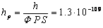 J·s. Due to the fact that different levels of matter
have different corresponding Planck constants and different energies of
emission of corresponding quanta, at each level of matter the ratio for the
energy of electromagnetic quantum
J·s. Due to the fact that different levels of matter
have different corresponding Planck constants and different energies of
emission of corresponding quanta, at each level of matter the ratio for the
energy of electromagnetic quantum  must contain
its own Planck constant. Thus, at the level of praons the quantum energy is
must contain
its own Planck constant. Thus, at the level of praons the quantum energy is  , where
  is the quantum
frequency. The next lower level of matter
is the graon level, while the graon is related to the praon, just as the praon is related to the proton.
is the quantum
frequency. The next lower level of matter
is the graon level, while the graon is related to the praon, just as the praon is related to the proton.
Let us turn
our attention to on the length of free path of gravitons. In cosmic space,
according to the findings of Lambda-Cold Dark Model ( ), the critical mass density reaches the value
 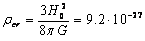 kg/m3,
if we assume that the Hubble constant
kg/m3,
if we assume that the Hubble constant  is 70 km/(s·Mpc) [21]. The physical density of the visible baryon
matter is
is 70 km/(s·Mpc) [21]. The physical density of the visible baryon
matter is  kg/m3,
which gives the concentration of
kg/m3,
which gives the concentration of  nucleons per
cubic meter. From the ratio at a given concentration
of nucleons and the value according to (18) we find the length
of free path of gravitons:
nucleons per
cubic meter. From the ratio at a given concentration
of nucleons and the value according to (18) we find the length
of free path of gravitons:  m. This value is 23 orders of magnitude greater than
the apparent size of the Universe, which is estimated as 14 billion parsecs or
m. This value is 23 orders of magnitude greater than
the apparent size of the Universe, which is estimated as 14 billion parsecs or  m. Consequently, gravitons can get into our visible
Universe from outside.
m. Consequently, gravitons can get into our visible
Universe from outside.
From the
standpoint of similarity of matter levels, the set of all stars in the visible
Universe corresponds to extremely rarefied atomic gas.
At first glance, this rarefied gas of stars, even in view of the lower levels
of matter, cannot create this energy density of the graviton field  J/m3, which we have found in (19). But in
remote areas of cosmic space the density of matter can be much greater and
reach such values, that it can generate the necessary energy density of the graviton
field, reaching our Universe.
J/m3, which we have found in (19). But in
remote areas of cosmic space the density of matter can be much greater and
reach such values, that it can generate the necessary energy density of the graviton
field, reaching our Universe.
In [17] we
explained the effects of red shift of the galaxy spectra and the attenuation of
emission from distant supernovae by the fact that the light is scattered on new
particles. These particles are neutral particles of muon type, which emerged
naturally in the same way as white dwarfs emerge in the course of stellar
evolution. The sizes of new particles and their concentration in space,
according to the theory of infinite nesting of matter, are so just such that can
explain the scattering of light. New particles also explain the appearance of
background emission and the effects attributed to dark matter. If we admit the
existence of new particles, then the most important arguments in favor of the
Big Bang model become useless. We are not limited by time period of 13.8
billion years as the age of the Universe. If the Universe has existed longer
than this time, then gravitons could have got into our Universe from outside
and carried out their action here.
6. THE ORIGIN
OF THE MASS
Let us
consider the energy density of the graviton field inside the body and near it.
Suppose there is a body in the form of a cube with an edge . The number of gravitons  per unit time
through a unit area during gravitons’ motion in the matter decreases according
to formula (2). During time six fluxes of
gravitons from each side will pass inside the cube through the faces with the
area
per unit time
through a unit area during gravitons’ motion in the matter decreases according
to formula (2). During time six fluxes of
gravitons from each side will pass inside the cube through the faces with the
area  and will change
up to the value:
and will change
up to the value:
 ,
,  ,
,
where  is the number
of gravitons that passed through the cube.
is the number
of gravitons that passed through the cube.
If gravitons
flew through the same empty volume, the number of gravitons coming out would be  . Consequently, the number of gravitons, which
interacted with the matter, equals:
. Consequently, the number of gravitons, which
interacted with the matter, equals:

Let us
assume that all these gravitons did not just transfer their momentum to the
matter and created the force of gravitation, but also transferred all their
energy to the matter. Then for the energy density in view of (16) we obtain:
 .
(27)
.
(27)
If the
neutron star has the radius 12 km and the mass 1.35 Solar
masses, then the average concentration of nucleons will be  m-3. Using (18-19) and assuming
 , we find
  and
and  J/m3.
Thus, if the gravitons interacting with the matter would transfer not only the
momentum but also their energy to it, the density of this energy would reach
the enormous value
J/m3.
Thus, if the gravitons interacting with the matter would transfer not only the
momentum but also their energy to it, the density of this energy would reach
the enormous value  in a short time
 s. Since we
cannot imagine that the neutron star could accumulate such amounts of energy, then
we should assume that although the gravitons transfer their momentum to the
stellar matter, but almost all their energy must be re-emitted back. If we
multiply in (27) by the
star’s volume and divide by the time
s. Since we
cannot imagine that the neutron star could accumulate such amounts of energy, then
we should assume that although the gravitons transfer their momentum to the
stellar matter, but almost all their energy must be re-emitted back. If we
multiply in (27) by the
star’s volume and divide by the time  , we will obtain the estimate of the graviton luminosity
of the star as the rate of the energy flux of the gravitons, interacting with
the stellar matter:
, we will obtain the estimate of the graviton luminosity
of the star as the rate of the energy flux of the gravitons, interacting with
the stellar matter:  W.
W.
In nature
there are many processes, in which the energy falling on bodies is almost
completely reflected or scattered without heating up the bodies. One of the
examples is the mirror, which receives the momentum of photons and reflects it
back with the same energy. Another example is the heating of planets by the Sun
– no matter how much the Sun is
emitting, all the light energy falling on the planets’ surface is eventually
emitted back into the space. But the closer a planet is to the Sun, the greater
energy flux falls on it and the higher is the temperature of the planet’s
surface and of its atmosphere. Since the graviton field is the same everywhere,
so wherever the body is located, the temperature inside the body, which arises
as a consequence of transformation of the energy of graviton fluxes, will be
unchanged, if the body’s parameters do not change. Apparently, the temperature
of graviton fluxes does not exceed the maximum temperature, which corresponds
to the virial theorem that connects the internal (thermal) energy of the
massive body and its gravitational energy.
From (27) we
will calculate the graviton luminosity of a body in the form of a cube,
multiplying by the volume  and dividing by
the time . Expressing the concentration of nucleons in terms of
the mass, in view of (16) we have:
and dividing by
the time . Expressing the concentration of nucleons in terms of
the mass, in view of (16) we have:
 ,
,  . (28)
From (28) it
follows that the graviton luminosity of the body  , understood as the luminosity of those graviton
fluxes that interacted with the matter and gave their momentum to it, is
proportional to body mass . This means that the mass, as a measure of body’s
inertia, can be expressed in terms of the parameters of the graviton fluxes
interacting with the body. The more gravitons transfer their momentum to the
body per unit time, the greater is the mass and inertia of the body and the
greater force is required to accelerate the body.
, understood as the luminosity of those graviton
fluxes that interacted with the matter and gave their momentum to it, is
proportional to body mass . This means that the mass, as a measure of body’s
inertia, can be expressed in terms of the parameters of the graviton fluxes
interacting with the body. The more gravitons transfer their momentum to the
body per unit time, the greater is the mass and inertia of the body and the
greater force is required to accelerate the body.
In (28)
there is a product  equal to the number
of nucleons in the body under consideration. Then the graviton luminosity per one nucleon, in view of (16), will equal:
equal to the number
of nucleons in the body under consideration. Then the graviton luminosity per one nucleon, in view of (16), will equal:
 W. (29)
The ratio of
the luminosity  to the average
energy of a graviton gives the
number of gravitons that interact with one nucleon of matter per unit time and
gave their momentum to it. According to (29), this number of gravitons is equal
to the product
to the average
energy of a graviton gives the
number of gravitons that interact with one nucleon of matter per unit time and
gave their momentum to it. According to (29), this number of gravitons is equal
to the product  , while the cross-section characterizes
the effective area of nucleon’s interaction with gravitons, and the coefficient
6 is associated with the six sides of cubic distribution of graviton fluxes in (2).
, while the cross-section characterizes
the effective area of nucleon’s interaction with gravitons, and the coefficient
6 is associated with the six sides of cubic distribution of graviton fluxes in (2).
We can also
substitute the quantity from (18) into (28):
 .
.
This relation
shows that the graviton luminosity is proportional and almost equal to the rest
energy of the body, released from the body per time as the time of gravitons’
passing the radius of the body. On the one hand, it is the consequence of
determining the cross-section of gravitons’
interaction with the matter in (18). On the other hand, the influence of strong
gravitation at the level of atoms leads to the fact that the characteristic
speed of the nucleons’ matter is equal to the speed of light. Besides,
according to (23) the total energy of a nucleon, which is approximately
estimated as half of its energy in the field of strong gravitation, is equal by
its absolute value to the rest energy as the product of mass and the squared
speed of light. In nuclear reactions with nucleons part of the rest energy is
released, and based on the above-mentioned we have every reason to believe that
this energy results from the energy of the graviton field acting at the atomic
level of matter.
7. CONCLUSION
The expressions
for the gravitational field strengths inside the ball (8) and outside (15),
obtained in the model of gravitons, are in good agreement with the values of
the field strengths in the Lorentz-invariant theory of gravitation. From the
field strengths we can easily proceed to the scalar potentials of the
gravitational field, since the strength is up to a sign determined as the
potential gradient. The field’s scalar potential is found up to an integration
constant by the contour integral of the field strength, taken along some path.
In this case, the potential specifies the energy of unit mass in the
gravitational field, which can be seen from the fact that the strength in the
contour integral is the gravitational force calculated per unit mass.
As long as
the matter density is less than the matter density of neutron stars, the
superposition principle will hold for the formulas of the field strengths and
potentials, according to which the strength or the potential of the system of
particles is equal to the sum of the corresponding values of individual
particles. As it was shown in [22], applying the superposition principle and
the method of retarded potentials to the system of point particles inside the
sphere leads to the formulas, according to which the gravitational potential of
the system looks as if it emerges from a single particle with the mass, equal
to the total mass of particles in this system, which is located in the center
of the system. The formulas obtained further are transformed using Lorentz
transformations in accordance with the Lorentz-invariant theory of gravitation.
Once we find
the gravitational scalar potential, then with the help of a special procedure
[23] in the framework of the Covariant Theory of Gravitation we can find the
4-potential, the stress-energy tensor of the gravitational field, the
gravitational field equations, the gravitational force, as well as the
contribution of the gravitational field into the equation for the metric. This
means that the gravitational field theory both in the flat Minkowski space and
in the curved spacetime is fully proved at the substantial level through the
graviton field. And the dependence of metric on the gravitational field
potential allows us to take into account the influence of the inhomogeneous
graviton field on the results of space-time experiments, based as a rule on the
use of electromagnetic waves and devices.
We can use also axiomatic approach to General Relativity which is described
in [24], for derivation of the geodesic
equation and other equations. The Newtonian theory of gravitation is a base for
the General Relativity since we can calibrate the metric derived from Einstein
equations choosing the low field limit and approximation of the classical law
of universal gravitation.
The
Covariant Theory of Gravitation and General
Relativity are both the metric theories. The main difference between them is
that in the Covariant Theory of Gravitation the gravitation is a real fundamental force and in General Relativity the
gravitation is replaced by action of metric field. In both theories the metric
should describe some phenomena such as gravitational dilation, gravitational
redshift and so on, which are seen as corrections to results of the Newtonian
theory of gravitation.
In (19) we
made an estimate of the energy density of the graviton field, in (18) we
presented the cross-section of gravitons’ interaction with the matter, in (20)
we estimated the rate of the energy flux of the graviton field in one
direction, in (21) we obtained the temperature  K of the
graviton field in the form of photons. The generalized temperature at the center
of a typical neutron star and a proton is apparently less than the temperature
of the graviton field, as a consequence of the fact that these objects do not
completely absorb the graviton fluxes. Based on the principles of the theory of
infinite nesting of matter, the densest objects at each level of matter are
assumed as the sources of the graviton field – neutron stars and magnetars, nucleons and atoms,
praons as the components that make up nucleons, etc. These objects emit
neutrinos, photons and high-energy cosmic rays that can make contribution to
the graviton field at all levels of matter.
K of the
graviton field in the form of photons. The generalized temperature at the center
of a typical neutron star and a proton is apparently less than the temperature
of the graviton field, as a consequence of the fact that these objects do not
completely absorb the graviton fluxes. Based on the principles of the theory of
infinite nesting of matter, the densest objects at each level of matter are
assumed as the sources of the graviton field – neutron stars and magnetars, nucleons and atoms,
praons as the components that make up nucleons, etc. These objects emit
neutrinos, photons and high-energy cosmic rays that can make contribution to
the graviton field at all levels of matter.
For
comparison, recent experiments at relativistic ion collider in Brookhaven have
shown [25] that nucleon
matter can be heated in collisions up to  K. In this case, the nucleon matter
behaves similarly to a liquid with very low viscosity, and its temperature is
less than the temperature of the graviton field.
K. In this case, the nucleon matter
behaves similarly to a liquid with very low viscosity, and its temperature is
less than the temperature of the graviton field.
In the
theory of infinite nesting of matter, the sequence of matter levels is as
follows: the level of graons – the level of praons – the level of nucleons – the level of neutron stars – and so on, both decreasingly and increasingly from the
point of view of mass of the main object
at a given matter level. Each level of matter is characterized by its
own gravitation and its own constant, which is similar in meaning to the Planck
constant. Ordinary gravitation is manifested most of all at the level of
planets and stars, and we suppose that the gravitons for ordinary gravitation
are the particles of the praon level of matter, located two levels below the
level of stars, which acquired their energy in relativistic processes near
nucleons. Strong gravitation is acting at the level of nucleons, and reasoning
by analogy, the gravitons for strong gravitation should be the particles of the
graon level of matter, which acquired their energy in processes near praons.
The gravitons can be both neutral particles, such as neutrinos and photons, and
relativistic charged particles, similar in their properties to cosmic rays. The
effective mass of all these particles is their relativistic mass-energy, taking
into account the great in magnitude Lorentz factor. In particular, the
gravitons can be the praons accelerated by the strong fields near nucleons
almost to the speed of light. As part of the graviton field, such relativistic
praons can participate in creation of ordinary gravitation, according to the Le
Sage’s model, and give mass to the bodies at the macrolevel.
In this case, the praons have their own rest mass, which arises from the action
of the gravitons of lower levels of matter. During interaction with the fields
and the matter, relativistic praons can produce high-energy photons, which can
also serve as the particles of the graviton field. The energy of ordinary
photons is proportional to their frequency and the Planck constant. But for the
particles belonging to different levels of matter, the value of the Planck
constant varies considerably according to the infinite nesting of matter – the
lower is the level of matter, the less is the respective Planck constant and
the lower is the energy of photons at this level of energy. As a result, the
graviton field represents a multi-component system of particles, photons and
neutrinos, the energies of which are associated with each of an infinite number
of matter levels.
In formula
(28) we expressed the body mass in terms of the luminosity of those graviton fluxes
that interacted with the body matter and transferred their momentum to it. The
body mass at a constant volume is proportional to the concentration of
nucleons, and similarly the number of interactions of gravitons with nucleons
increases with increasing of concentration of nucleons. Thus, the body’s
inertia as the resistance to the applied force and gravitational mass of the
body are caused by the action of the graviton field on the given body. As it follows from the principle of relativity, at a constant
velocity the action of graviton fluxes from different sides is balanced, but it
is not so in case of the body’s acceleration. When the body is
accelerated, a force must be applied and work must be carried out to bring the
body from the state with one velocity into the state with a different velocity.
This work is done against the action of gravitons fluxes and leads to the
concept of mass as a measure of the body’s inertia proportional to the applied
force and inversely proportional to the emerging acceleration. In this case the
main contribution to the bodies’ inertia is made by the graviton field at the
atomic level, where there is strong gravitation.
We should
also note the difference in how we understand the concept of the graviton
field. In our approach, the graviton field is the source of gravitational
force, it exists as a necessary addition to the matter in the form of
elementary particles and bodies composed of them, it creates these bodies in
the processes of gravitational clustering of scattered matter, and is generated
due to the emission from the densest objects, such as graons,
praons, nucleons and neutron stars.
In contrast,
in the quantum theory of gravitation the concept of a graviton field is
maximally reduced to such a graviton field, to which any gravitational wave
corresponds. Such gravitons are attributed, by analogy with the electromagnetic
wave and photons, the dependence of the graviton energy on the Planck constant  and on the
frequency of the gravitational wave
and on the
frequency of the gravitational wave  . In our opinion, this approach could be erroneous, especially
if we take into account that most part of gravitons can be generated not at the
level of atoms, but at a lower level of matter, where the Planck constant
should be replaced with some other similar constant. On the other hand,
considering the elementary process of emission in the hydrogen atom shows [5],
that together with the electromagnetic quantum, during transition of an
electron from a certain energy level to a lower level, the atom produces
quadrupole emission of the gravitational quantum with the energy
. In our opinion, this approach could be erroneous, especially
if we take into account that most part of gravitons can be generated not at the
level of atoms, but at a lower level of matter, where the Planck constant
should be replaced with some other similar constant. On the other hand,
considering the elementary process of emission in the hydrogen atom shows [5],
that together with the electromagnetic quantum, during transition of an
electron from a certain energy level to a lower level, the atom produces
quadrupole emission of the gravitational quantum with the energy  , which depends not only on the Planck constant, but
also on the electron’s velocity and on the
ratio of the electron mass to the proton mass
, which depends not only on the Planck constant, but
also on the electron’s velocity and on the
ratio of the electron mass to the proton mass  . It implies the difference of processes of emission
of electromagnetic and gravitational quanta at the atomic level, as well as the
difference of processes of absorbing these quanta.
. It implies the difference of processes of emission
of electromagnetic and gravitational quanta at the atomic level, as well as the
difference of processes of absorbing these quanta.
In the
General Relativity, two bodies rotating near each other, emit a quadrupole
gravitational wave. From the standpoint of the Covariant Theory of Gravitation
[5], each body produces mainly dipole emission, but in the total emission of
the system the dipole components are canceled and only the quadrupole component
is left. The gravitational wave carries the energy and angular momentum away
from the system. This happens because during rotation the bodies have a
time-varying centripetal acceleration and the bodies carry out work against the
graviton fluxes, when their angular momentum is reduced. As a rule, the energy
of the gravitational wave is equal to the change in the total energy of the
system in the form of two bodies. Obviously, such a gravitational wave is just
a ripple on the graviton field, which is involved in producing the
gravitational force between the bodies of the system. Accordingly, the
gravitons of this wave, if we artificially separate them with the help of the Planck
constant as portions of the gravitational energy, can have nothing in common
with real gravitons, which produce the graviton field in our model.
REFERENCES
1.
Fatio de Duillier, N.
(1701), Die wiederaufgefundene
Abhandlung von Fatio de Duillier: De la cause de la Pesanteur, in Bopp, Karl, "Drei
Untersuchungen zur
Geschichte der Mathematik", Schriften der Straßburger
Wissenschaftlichen Gesellschaft
in Heidelberg (Berlin & Leipzig,
published 1929) 10: 19–66.
2.
Georges-Louis Le Sage (1756), "Letter à une académicien de Dijon..", ercure de France:
153–171.
3.
Ritz W. Recherches
critiques sur l'Électrodynamique
générale. Ann. de chim. et phys., 13, 1908.
4.
C. W. Misner, K. S. Thorne, and J. A. Wheeler, Gravitation (W. H. Freeman, San
Francisco, CA, 1973).
5.
Sergey Fedosin, The physical theories and infinite hierarchical
nesting of matter, Volume 1, LAP LAMBERT Academic Publishing, pages: 580, ISBN-13:
978-3-659-57301-9.
6.
Fedosin S.G. Sovremennye problemy fiziki: v poiskakh novykh printsipov. Moskva: Editorial
URSS, 2002, 192 pages. ISBN 5-8360-0435-8.
7.
Fedosin S.G. Model of Gravitational Interaction in the
Concept of Gravitons. Journal of
Vectorial Relativity, 2009, Vol. 4, No. 1, P. 1 – 24.
8.
Fedosin S. G. Fizika i filosofiia podobiia ot
preonov do metagalaktik. (Perm, 1999). ISBN 5-8131-0012-1.
9.
Rothman, T.; Boughn,
S. (2006). Can Gravitons be Detected? Foundations of
Physics, 36 (12): 1801–1825. doi:10.1007%2Fs10701-006-9081-9 .
10.
Freeman Dyson. Is a Graviton Detectable? Poincare Prize Lecture, International Congress of Mathematical Physics,
Aalborg, Denmark, August 6, 2012.
11.
Maurizio Michelini. A Flux of Micro Quanta Explains Relativistic
Mechanics and the Gravitational Interaction. Apeiron. 2007, Vol. 14, No 2, P. 65-94.
12.
Fedosin S.G. Electromagnetic and Gravitational Pictures of the World. Apeiron, 2007, Vol. 14, No. 4, P. 385 – 413.
13.
Kiefer, C.; Weber, C. On the interaction of mesoscopic quantum systems
with gravity. Annalen der Physik, 2005, Vol.
14, Issue 4, Pages 253 – 278.
14.
Fedosin S.G. Scale Dimension as the Fifth Dimension of
Spacetime. Turkish Journal of Physics, 2012, Vol. 36,
No 3, P. 461 – 464. doi:
10.3906/fiz-1110-20.
15.
Fedosin S.G. The Integral Energy-Momentum 4-Vector and
Analysis of 4/3 Problem Based on the Pressure Field and Acceleration Field. American Journal of Modern Physics. Vol.
3, No. 4, 2014, pp. 152-167. doi:
10.11648/j.ajmp.20140304.12.
16.
Fedosin S.G. The radius of the proton in the self-consistent
model. Hadronic Journal, 2012, Vol. 35, No. 4, P. 349 – 363.
17.
Fedosin S.G. Cosmic Red Shift, Microwave Background, and New Particles. Galilean Electrodynamics, 2012, Vol. 23, Special Issues No. 1, P. 3 – 13.
18.
Alexander Y. Potekhin, Andrea De Luca and Jose A.
Pons. Neutron Stars – Thermal Emitters. arXiv:1409.7666. Accepted by Space Science
Reviews.
19.
Piotr Homola.
Ultra-high energy photon studies with the Pierre Auger Observatory. Proceedings
of the 31st International Cosmic Ray Conference, Lod´z, Poland, 2009.
20.
Javier Tiffenberg. Limits on the diffuse flux of
ultra high energy neutrinos set using the Pierre Auger Observatory. Proceedings
of the 31st International Cosmic Ray Conference, Lod´z, Poland, 2009.
21.
Hinshaw, G.F., et.al. Nine-Year Wilkinson Microwave Anisotropy Probe (WMAP)
Observations: Cosmological Parameter Results. ApJS., 2013, Vol. 208, 19H.
22.
Fedosin S.G. 4/3 Problem for the Gravitational Field. Advances in Physics Theories and Applications, 2013, Vol. 23, P. 19 – 25.
23.
Fedosin S.G. The Procedure of Finding the
Stress-Energy Tensor and Equations of Vector Field of Any Form. Advanced Studies in Theoretical Physics, Vol.
8, 2014, no. 18, 771 – 779. doi: 10.12988/astp.2014.47101.
24.
Fedosin S.G. The General Theory of Relativity, Metric Theory of
Relativity and Covariant Theory of Gravitation: Axiomatization and Critical
Analysis. International Journal of Theoretical and Applied Physics (IJTAP), 2014,
Vol. 4, No. 1, P. 9 – 26.
25.
'Perfect' Liquid Hot Enough to be Quark Soup. Brookhaven
National Laboratory News, 2010.
Source: http://sergf.ru/fgen.htm
Scientific site