Canadian Journal of Physics,
Vol. 94, No. 4, P. 370-379 (2016). http://dx.doi.org/10.1139/cjp-2015-0593
Estimation of the physical parameters
of planets and stars in the gravitational equilibrium model
Sergey G. Fedosin
Sviazeva
Str. 22-79, Perm, 614088, Perm region, Russian Federation
e-mail
intelli@list.ru
Abstract: The motion equations of matter in
the gravitational field, acceleration field, pressure field and other fields
are considered based on the field theory. This enables us to derive
simple formulas in the framework of the gravitational equilibrium model, which
allow us to estimate the physical parameters of cosmic bodies. The acceleration
field coefficient ![]() and the pressure field coefficient
and the pressure field coefficient ![]() are a function of the state of matter, and
their sum is close in magnitude to the gravitational constant
are a function of the state of matter, and
their sum is close in magnitude to the gravitational constant
![]() . In the
presented model the dependence is found of the internal temperature and
pressure on the current radius. The central temperatures and pressures are calculated
for the Earth and the Sun, for a typical neutron star and a white dwarf. The
heat flux and the thermal conductivity coefficient of the matter of these
objects are found, and the formula for estimating the entropy is provided. All
the quantities are compared with the calculation results in different models of
cosmic bodies. The discovered good agreement with these data proves the
effectiveness and universality of the proposed model for estimating the
parameters of planets and stars and for more precise calculation of physical
quantities.
. In the
presented model the dependence is found of the internal temperature and
pressure on the current radius. The central temperatures and pressures are calculated
for the Earth and the Sun, for a typical neutron star and a white dwarf. The
heat flux and the thermal conductivity coefficient of the matter of these
objects are found, and the formula for estimating the entropy is provided. All
the quantities are compared with the calculation results in different models of
cosmic bodies. The discovered good agreement with these data proves the
effectiveness and universality of the proposed model for estimating the
parameters of planets and stars and for more precise calculation of physical
quantities.
Keywords: field theory; acceleration field; pressure
field; gravitational field; gravitational equilibrium model.
PACS: 03.30.+p, 03.50.-s, 03.65.pm,
04.40.-b, 95.30.Sf
Résumé: Sur la base de la théorie
des champs les équations du mouvement
de la matière dans le champ
gravitationnel, le champ de l'accélération,
le champ de pression et dans
autres champs sont considérées. Cela permet de dériver
dans le domaine du modèle d'équilibre gravitationnel des formules
simples qui permettent de faire des estimations des paramètres physiques des corps spatiaux.
Le coefficient du champ de l'accélération ![]() et le coefficient du champ de pression
et le coefficient du champ de pression ![]() sont une fonction de l'état de la matière, et leur somme est
proche en amplitude à la constante
gravitationnelle
sont une fonction de l'état de la matière, et leur somme est
proche en amplitude à la constante
gravitationnelle ![]() . Dans le présent modèle, les dépendances de
temperature et pression intérieures du rayon actuel sont trouvées. Les températures centrales et les pressions sont calculées pour la Terre et
le Soleil, pour une étoile
à neutrons typique et une naine blanche. Le flux thermique et le coefficient de conductivité thermique de la matière de ces objets sont
trouvés et une formule d'estimation de l'entropie est présentée. Toutes les quantités sont
comparées avec les résultats
des calculs en les différents
modèles de corps spatiaux.
Une bonne conformité trouvée avec les données confirme l'efficacité et l'universalité du
modèle proposé pour estimer les paramètres des planètes et des étoiles, et pour les calculs plus
précis de quantités physiques.
. Dans le présent modèle, les dépendances de
temperature et pression intérieures du rayon actuel sont trouvées. Les températures centrales et les pressions sont calculées pour la Terre et
le Soleil, pour une étoile
à neutrons typique et une naine blanche. Le flux thermique et le coefficient de conductivité thermique de la matière de ces objets sont
trouvés et une formule d'estimation de l'entropie est présentée. Toutes les quantités sont
comparées avec les résultats
des calculs en les différents
modèles de corps spatiaux.
Une bonne conformité trouvée avec les données confirme l'efficacité et l'universalité du
modèle proposé pour estimer les paramètres des planètes et des étoiles, et pour les calculs plus
précis de quantités physiques.
Les mots-clés: la théorie du champ, le champ d’accélération,
le champ de pression, le champ gravitationnel,
modèle d’équilibre gravitationnel.
1. Introduction
The most accurate models
of cosmic objects include detailed numerical calculations of certain internal
structures (the solid or liquid core, shell, convective zone) with the use of
equations of the state of different phases of matter and acting fields. For
compact objects it is necessary to take into account the quantum and
relativistic effects.
However, physics has in
store the models that allow us to quickly estimate the characteristic
parameters of planets and stars based only on the observable data, such as
radius, luminosity, spectrum, surface temperature, gravitational redshift,
asteroseismology data, etc. A well-known example is a polytropic model, in
which the gas pressure is related to the mass density by a polytrope at the
constant thermal capacity of the matter [1-3]. With polytropic
index ![]() and
and ![]() the model gives the correct order of such
quantities as the central density, temperature, pressure, potential
gravitational energy and a number of other quantities.
the model gives the correct order of such
quantities as the central density, temperature, pressure, potential
gravitational energy and a number of other quantities.
White dwarfs are
objects, in which the electron gas degenerates and makes the major contribution
to the pressure in the matter. For neutron stars, the same is true for the
neutron gas. There is a well-known simple calculation of the state of matter in
white dwarfs and neutron stars, based on the equality of the gravitational
energy and quantum mechanical energy and providing the typical values of the
masses and radii of these objects. A more detailed analysis leads to the
Chandrasekhar limit [4-5] as the greatest mass of a white dwarf, beyond which
it becomes a neutron star.
In [6] the structure of
compact stars is modeled by solving the equation of hydrostatic equilibrium by
parameterization of the mass density dependence on the radius. This leads to
the dependence of the masses and radii of the objects on the central density
and the dependence of the pressure on the radius, expressed in terms of the
gamma-function and the hypergeometric function.
The natural drawbacks of
the above-mentioned approaches are the limited range of application or the low
accuracy of predictions of physical quantities and the internal structure of
objects.
Next, we will present
the model of gravitational equilibrium, which is based on the field theory. In
order to illustrate the possibilities of this model, we will calculate some
physical parameters of a number of objects and will compare them
with the results of calculations made by other authors. The positive aspect of
the proposed approach is its universality, which allows applying it to any
cosmic objects. In addition, this model provides very simple formulas to
estimate the parameters of planets and stars at minimum of necessary
assumptions.
2. The model description
In the model of
gravitational equilibrium it is assumed that the corresponding object (planet,
star) is in a state when the processes of energy exchange between the
gravitational field and other fields have finished in it. From a theoretical
point of view, all the fields acting in cosmic objects can be viewed as the components
of a single general field [7]. In addition to the gravitational field, which is
the main component, contribution to the general field can also be made by the
electromagnetic field, pressure field, acceleration field, dissipation field,
strong interaction field, weak interaction field, as well as other fields in
the matter of the objects under consideration. At equilibrium, all the fields
are relatively independent, because the energy fluxes between the fields and
the matter on the average tend to zero. The expression for the general field
equations follows from the principle of least action:
![]() ,
, ![]() , (1)
, (1)
where ![]() is the general field tensor,
is the general field tensor,
![]() is the general field coefficient,
is the general field coefficient,
![]() is the Levi-Civita symbol or completely
antisymmetric unit tensor,
is the Levi-Civita symbol or completely
antisymmetric unit tensor,
![]() is the mass four-current,
is the mass four-current,
![]() is the mass density in the reference frame associated with the particle,
is the mass density in the reference frame associated with the particle,
![]() is the four-velocity of a point particle,
is the four-velocity of a point particle, ![]() is the speed of light.
is the speed of light.
Since the general field
tensor is the sum of tensors of particular fields, then
the equations of any field can be represented in the form of (1) after the
respective substitution of the field tensor, the constant of this field and the
four-current. A characteristic feature of (1) is the fact that the equations of
the general field and of each particular field have the form of Maxwell
equations for the electromagnetic field, written in a covariant form in the
curved space for non-inertial reference frames.
3. The acceleration field and the temperature
The equations of the acceleration
field according to (1) have the following form [8]:
![]() ,
, ![]() , (2)
, (2)
where ![]() is the acceleration field tensor,
is the acceleration field tensor, ![]() is the acceleration field coefficient.
is the acceleration field coefficient.
The tensor ![]() includes the vector components
includes the vector components ![]() and
and ![]() , which can be
found by the rule:
, which can be
found by the rule:
![]() ,
, ![]() , (3)
, (3)
where the indices ![]() form a triples of non-recurring numbers of the
form 1,2,3 or 3,1,2 or 2,3,1; the three-vectors
form a triples of non-recurring numbers of the
form 1,2,3 or 3,1,2 or 2,3,1; the three-vectors ![]() and
and ![]() can be expanded into the components:
can be expanded into the components: ![]() ;
; ![]() .
.
For simplicity, we will consider equations (2) in the flat Minkowski
space, that is, within the framework of the special theory of relativity. In
this case, equations (2) are written as the equations for strength ![]() and for the solenoidal vector
and for the solenoidal vector ![]() of the acceleration field:
of the acceleration field:
![]() ,
, ![]() ,
, ![]() ,
, ![]() . (4)
. (4)
With the help of the vectors ![]() and
and ![]() we can form an acceleration four-vector,
characteristic of the body particles moving at the velocity
we can form an acceleration four-vector,
characteristic of the body particles moving at the velocity ![]() and having the Lorentz factor
and having the Lorentz factor ![]() :
:
![]() ,
,
![]() .
(5)
.
(5)
A gravitationally bound body usually has a spherical shape, so that the
four-acceleration ![]() with a covariant index will be a certain
coordinate function. The vectors
with a covariant index will be a certain
coordinate function. The vectors ![]() and
and ![]() also allow us to calculate the stress-energy
tensor of the acceleration field
also allow us to calculate the stress-energy
tensor of the acceleration field ![]() and the vector
and the vector ![]() ,
which is the vector of the energy-momentum flux density of the acceleration
field.
,
which is the vector of the energy-momentum flux density of the acceleration
field.
The main reason that the acceleration field of the matter particles has
its own energy density, energy flux density and field strength is the
gravitation force. Under the action of this force the gradients of pressure,
temperature, mass density and other quantities are formed in cosmic bodies. The
closer to the center of the body we approach, the higher the temperature and, consequently,
the average velocity of the particles and the value of the four-velocity
become. For a single particle, the four-potential of the acceleration field is
the covariant four-velocity ![]() of this particle. However, in case of a set of
closely interacting particles it is not so – in the total four-potential of the
system’s acceleration field
of this particle. However, in case of a set of
closely interacting particles it is not so – in the total four-potential of the
system’s acceleration field ![]() the scalar potential
the scalar potential ![]() and the vector potential
and the vector potential ![]() of the acceleration field become independent
quantities as a consequence of different rules of summation of contributions
from the scalar and vector quantities of different particles.
of the acceleration field become independent
quantities as a consequence of different rules of summation of contributions
from the scalar and vector quantities of different particles.
In [9], we calculated the energy and the vector of the energy-momentum
flux density ![]() of the acceleration field for a set of
similarly charged particles that form a gravitationally bound system in the
form of some liquid and filling a spherical volume. The same was done for other
fields, including the gravitational and electromagnetic fields, as well as the
pressure field. It allowed estimating the acceleration field coefficient in a
first approximation with the help of the gravitational constant
of the acceleration field for a set of
similarly charged particles that form a gravitationally bound system in the
form of some liquid and filling a spherical volume. The same was done for other
fields, including the gravitational and electromagnetic fields, as well as the
pressure field. It allowed estimating the acceleration field coefficient in a
first approximation with the help of the gravitational constant
![]() , the vacuum
permittivity
, the vacuum
permittivity ![]() and the relation
and the relation ![]() for the particles in question:
for the particles in question:
![]() .
(6)
.
(6)
In article [10], the
concept of acceleration field allowed us to calculate the relativistic energy
of the system of particles and the gravitational mass of the system; and in
[11] it allowed us to derive the relativistic Navier-Stokes equations for
viscous charged matter, taking into account the pressure field and dissipation
field.
Since in the definition ![]() the acceleration tensor is expressed in terms
of the four-potential of the acceleration field, in equations (2) we can pass
on from the acceleration tensor to the four-potential
the acceleration tensor is expressed in terms
of the four-potential of the acceleration field, in equations (2) we can pass
on from the acceleration tensor to the four-potential ![]() . This leads
to the wave equations for the potentials
. This leads
to the wave equations for the potentials ![]() and
and ![]() of the acceleration field [12]:
of the acceleration field [12]:
![]() . (7)
. (7)
In (7) ![]() is the four-potential of the acceleration
field, expressed with a contravariant index using the metric tensor
is the four-potential of the acceleration
field, expressed with a contravariant index using the metric tensor
![]() , and
, and ![]() are the Christoffel symbols, which are the
function of
are the Christoffel symbols, which are the
function of ![]() . We solved
equation (7) in [9] for the case of a set of randomly moving particles without
general rotation, which are connected with each other by means of gravitation
and the electromagnetic field including the pressure field. In Minkowski space
the scalar component (7) is reduced to the equation for the Lorentz factor,
thus we obtain the following:
. We solved
equation (7) in [9] for the case of a set of randomly moving particles without
general rotation, which are connected with each other by means of gravitation
and the electromagnetic field including the pressure field. In Minkowski space
the scalar component (7) is reduced to the equation for the Lorentz factor,
thus we obtain the following:
![]() ,
, ![]() ,
, ![]() , (8)
, (8)
where the Lorentz factor ![]()
is the function of the current radius ![]() inside the sphere and the average value for
the set of particles,
inside the sphere and the average value for
the set of particles, ![]() is the average velocity of the particles in the
reference frame
is the average velocity of the particles in the
reference frame ![]() , which is
associated with the center of inertia of the system.
, which is
associated with the center of inertia of the system.
The solution of (8) in
case of uniform density is the following expression:
 , (9)
, (9)
where ![]() is the Lorentz factor for the velocities
is the Lorentz factor for the velocities ![]() of the particle in the center of the sphere.
of the particle in the center of the sphere.
From (9) by raising to
the square we obtain approximately the following:
![]() ,
(10)
,
(10)
so that as the current radius ![]() inside the sphere increases while moving from
the center to the periphery of the sphere, the velocity
inside the sphere increases while moving from
the center to the periphery of the sphere, the velocity ![]() of the particles decreases.
of the particles decreases.
Assuming that the velocity ![]() is the root mean square velocity of the
particles, and taking into account its relation to the kinetic temperature in
the form of
is the root mean square velocity of the
particles, and taking into account its relation to the kinetic temperature in
the form of ![]() , where
, where ![]() is the Boltzmann constant, expression (10) is
transformed into the temperature-radius dependence:
is the Boltzmann constant, expression (10) is
transformed into the temperature-radius dependence:
![]() .
(11)
.
(11)
where ![]() is the temperature at the center of the
sphere,
is the temperature at the center of the
sphere, ![]() is the mass of one gas particle,
is the mass of one gas particle, ![]() is the mass within the current radius
is the mass within the current radius ![]() .
.
From (11) it follows
that the temperature inside the cosmic bodies in the first approximation
decreases parabolically, depending on the square of the radius of the
observation point. Assuming in (11) that at the body radius ![]() the body mass is equal to
the body mass is equal to ![]() , and
neglecting the surface temperature
, and
neglecting the surface temperature ![]() , we find
the formula for the temperature in the center of the body:
, we find
the formula for the temperature in the center of the body:
![]() .
(12)
.
(12)
4. The pressure field
The four-potential of
the pressure field for one particle is found by multiplying the function
depending on the pressure and density by the covariant four-velocity [8-9],
[12]:
![]() ,
(13)
,
(13)
where ![]() and
and ![]() denote the pressure and density in the
reference frame
denote the pressure and density in the
reference frame ![]() of the particle, the dimensionless ratio
of the particle, the dimensionless ratio ![]() is proportional to the pressure energy of the
particle per unit mass of the particle,
is proportional to the pressure energy of the
particle per unit mass of the particle, ![]() and
and ![]() are the scalar and vector potentials of the
pressure field.
are the scalar and vector potentials of the
pressure field.
For a system of
particles, (13) can also be considered valid, but ![]() should be considered not as the four-velocity
of an individual particle, but as the four-velocity averaged with respect to
some ensemble of particles near the observation point.
should be considered not as the four-velocity
of an individual particle, but as the four-velocity averaged with respect to
some ensemble of particles near the observation point.
The equations of the
pressure field according to (1) are as follows:
![]() ,
,
![]() , (14)
, (14)
where ![]() is the pressure field tensor,
is the pressure field tensor, ![]() is the pressure field coefficient.
is the pressure field coefficient.
The tensor ![]() is the result of applying the four-curl to the
four-potential
is the result of applying the four-curl to the
four-potential ![]() :
:
![]() , (15)
, (15)
 . (16)
here the tensor components are the
components of the strength vector ![]() and the solenoidal vector
and the solenoidal vector ![]() of the pressure field.
of the pressure field.
In Minkowski space,
equations of the pressure field (14) are considerably simplified:
![]() ,
, ![]() ,
, ![]() ,
, ![]() . (17)
. (17)
It is sufficient to know
the vectors ![]() and
and ![]() in order to determine the stress-energy tensor
in order to determine the stress-energy tensor ![]() , the vector
of the energy flux density
, the vector
of the energy flux density ![]() of the pressure field and the pressure force density
in the matter.
of the pressure field and the pressure force density
in the matter.
Substituting (15) into
(14) gives the wave equation for the four-potential of the pressure field:
![]() . (18)
. (18)
In case of a
self-gravitating system of particles without rotation, which occupies a
spherical volume, equation (18) and its solution for the scalar potential in
view of (9) is reduced to the following:
![]() .
(19)
.
(19)

Since there is a relation ![]() , at a constant
density the solution of (19) is transformed into the dependence of the pressure
inside the system:
, at a constant
density the solution of (19) is transformed into the dependence of the pressure
inside the system:
![]() .
(20)
.
(20)
In large cosmic bodies
the pressure on the surface at ![]() is rather low and we can neglect it in (20).
Then, to estimate the pressure in the center of the body we obtain a simple
formula:
is rather low and we can neglect it in (20).
Then, to estimate the pressure in the center of the body we obtain a simple
formula:
![]() .
(21)
.
(21)
5. The gravitational field and the
equation of motion of matter
The equations of the
gravitational field in the covariant theory of gravitation [13-16] correspond
in their form to (1):
![]() ,
, ![]() , (22)
, (22)
where ![]() is the gravitational field tensor, which
includes the components of the gravitational strength vector
is the gravitational field tensor, which
includes the components of the gravitational strength vector ![]() and the solenoidal vector
and the solenoidal vector ![]() of the torsion field:
of the torsion field:
 .
.
The starting point of
the covariant theory of gravitation is the four-potential of the gravitational field ![]() , which is
described by the field’s scalar potential
, which is
described by the field’s scalar potential ![]() and vector potential
and vector potential ![]() . The
four-potential is part of the Lagrangian and it allows us to derive the
equations of the gravitational field from the principle of least action, while
the field tensor is associated with the four-potential:
. The
four-potential is part of the Lagrangian and it allows us to derive the
equations of the gravitational field from the principle of least action, while
the field tensor is associated with the four-potential: ![]() .
This equality can be written in vector notation as follows:
.
This equality can be written in vector notation as follows:
![]() ,
, ![]() . (23)
. (23)
In Minkowski space, the
mass density ![]() , the mass
current density
, the mass
current density ![]() , the mass
four-current
, the mass
four-current ![]() , and
equations (22) have the following form:
, and
equations (22) have the following form:
![]() ,
, ![]() ,
, ![]() ,
, ![]() .
.
If in (22) we turn from
the tensor ![]() to the four-potential
to the four-potential ![]() , we will
obtain the wave equation:
, we will
obtain the wave equation:
![]() .
.
In Minkowski space, this equation falls into two equations for the potentials of the gravitational field:
![]() ,
, ![]() . (24)
. (24)
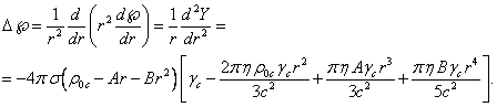
If the system of
particles does not move in space as a whole and has no general rotation, then
it has the vector potential ![]() and the torsion field
and the torsion field ![]() . And if the
potential
. And if the
potential ![]() does not depend on time, then the
gravitational field becomes static. In this case, according to [9], the scalar
potential inside the body at a constant mass density in view of (9) is defined
by the formula:
does not depend on time, then the
gravitational field becomes static. In this case, according to [9], the scalar
potential inside the body at a constant mass density in view of (9) is defined
by the formula:
 (25)
(25)
In the concept of the
general field [7] the equation of motion of matter is as follows:
 .
.
(26)
where ![]() is the four-acceleration in the curved space,
is the four-acceleration in the curved space, ![]() is the electromagnetic tensor,
is the electromagnetic tensor, ![]() is the electromagnetic four-current,
is the electromagnetic four-current, ![]() is the dissipation field tensor,
is the dissipation field tensor, ![]() is the strong interaction field tensor ,
is the strong interaction field tensor , ![]() is the weak interaction field tensor.
is the weak interaction field tensor.
The
tensors ![]() and
and ![]() are important in the cases,
when the equilibrium inside cosmic bodies is supported by the additional
pressure from thermonuclear reactions or radioactive decay. The vector component (26) in view of (5) is reduced to the following:
are important in the cases,
when the equilibrium inside cosmic bodies is supported by the additional
pressure from thermonuclear reactions or radioactive decay. The vector component (26) in view of (5) is reduced to the following:
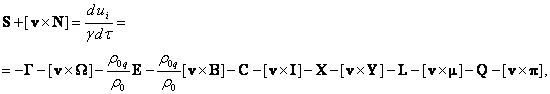 (27)
(27)
where the vectors ![]() ,
, ![]() and
and ![]() denote the strengths of the dissipation field,
strong interaction field and weak interaction field, respectively, and the
vectors
denote the strengths of the dissipation field,
strong interaction field and weak interaction field, respectively, and the
vectors ![]() ,
, ![]() and
and ![]() are the solenoidal vectors of these fields.
are the solenoidal vectors of these fields.
If we consider the
equation of motion in Minkowski space and take into account only the
gravitation, the
acceleration field and
the pressure field, then in the static case we can assume ![]() ,
, ![]() , and
, and ![]() . In view of (23) and (25) we have the following:
. In view of (23) and (25) we have the following:
![]() . (28)
. (28)
The pressure field
strength is given by the formula: ![]() , and if the
vector potential is
, and if the
vector potential is ![]() , then using
(19) we find the following:
, then using
(19) we find the following:
![]() . (29)
. (29)
According to (3) and the
definition of the acceleration field four-potential in the form of ![]() , the
acceleration field strength equals:
, the
acceleration field strength equals: ![]() .
.
For a non-rotating body
both the vector potential ![]() and the solenoidal vector
and the solenoidal vector ![]() are equal to zero. In this case, using (8-9) inside the body we find the following:
are equal to zero. In this case, using (8-9) inside the body we find the following:
![]() . (30)
. (30)
Substituting
![]() ,
, ![]() and
and ![]() in (27) in the absence of other fields, we
obtain the equality for the field strengths and the relation for the field
coefficients:
in (27) in the absence of other fields, we
obtain the equality for the field strengths and the relation for the field
coefficients:
![]() ,
, ![]() . (31)
. (31)
Outside the system, near
its border, we can assume that ![]() ,
, ![]() , and there
is a gravitational force acting on a certain test particle, but the pressure
tends to zero due to the low mass density. Then in (31) we should assume
, and there
is a gravitational force acting on a certain test particle, but the pressure
tends to zero due to the low mass density. Then in (31) we should assume ![]() , and the
gravitational field strength
, and the
gravitational field strength ![]() will determine the centripetal acceleration of
individual particles, rotating around the system. In the non-relativistic case,
this can be written as:
will determine the centripetal acceleration of
individual particles, rotating around the system. In the non-relativistic case,
this can be written as: ![]() . In view of
the equality
. In view of
the equality ![]() for the kinetic temperature of the particles
near the surface of the system we must obtain:
for the kinetic temperature of the particles
near the surface of the system we must obtain:
![]() . (32)
. (32)
The kinetic temperature ![]() refers to the kinetic energy of the particles
during their rotation around the system and it should exceed the average
temperature
refers to the kinetic energy of the particles
during their rotation around the system and it should exceed the average
temperature ![]() of the gas of these particles, which is the
measure of the gas thermal energy near the system.
of the gas of these particles, which is the
measure of the gas thermal energy near the system.
The best conditions for
(32) to hold must be in gas clouds, for example, in Bok globules, small dark
cosmic clouds of gas and dust. In [17] it was found that the radius of a
typical globule is 0.35 parsecs, the mass is 11 Solar
masses, and the recorded temperature of dust in some globules can reach 26 K.
Assuming in (32) that ![]() is equal to an atomic mass unit, we find the
temperature of particles on the surface for a typical globule:
is equal to an atomic mass unit, we find the
temperature of particles on the surface for a typical globule: ![]() K. If in (11) we assume
K. If in (11) we assume ![]() ,
, ![]() ,
, ![]() , and
taking into account equation (6) for
, and
taking into account equation (6) for ![]() , the
temperature in the center of the globule is of the order of 22 K, which is
close enough to the observations.
, the
temperature in the center of the globule is of the order of 22 K, which is
close enough to the observations.
Using (32) for the Earth
gives the kinetic temperature ![]() of about 2500 K, and for the Sun – about 7.7 million degrees. Such
temperatures are actually observed – at the Earth's ionosphere the thermal temperature
of about 2500 K, and for the Sun – about 7.7 million degrees. Such
temperatures are actually observed – at the Earth's ionosphere the thermal temperature
![]() is over 2000 K, and at the Solar
corona the average temperature is about 5 million degrees. Due to the action of
the Sun’s gravitation the particles are orbiting around the star for a long
time, almost without losing their energy. This solves the well-known coronal
heating problem, according to which a fast-moving heated gas should evaporate
quickly and the corona should rapidly cool down due the insufficient rate of
its heating from the photosphere. It is obvious that in this analysis of the
problem it is not taken into account that the particles can be fully retained
by the gravitational field of the Sun and rotate
around it. In addition, if the particles are always close to the Sun, they can
be heated for a long time due to solar flares and similar phenomena, finally
reaching the observed temperature of millions of degrees.
is over 2000 K, and at the Solar
corona the average temperature is about 5 million degrees. Due to the action of
the Sun’s gravitation the particles are orbiting around the star for a long
time, almost without losing their energy. This solves the well-known coronal
heating problem, according to which a fast-moving heated gas should evaporate
quickly and the corona should rapidly cool down due the insufficient rate of
its heating from the photosphere. It is obvious that in this analysis of the
problem it is not taken into account that the particles can be fully retained
by the gravitational field of the Sun and rotate
around it. In addition, if the particles are always close to the Sun, they can
be heated for a long time due to solar flares and similar phenomena, finally
reaching the observed temperature of millions of degrees.
However, we must limit
the use of formulas (31) and (32) due to their incompleteness, because along
with the motion of particles in solid bodies and stellar plasma, the main
contribution into the pressure is made by the interatomic forces, including the
electromagnetic forces of electric charges and the strong gravitation as the
component of strong interaction (in the gravitational model of strong
interaction [14]). These forces can significantly change the particle acceleration
in the equation of motion (27).
For an ideal solid body
there is no motion of particles inside the body, ![]() , and from
(31), in view of (28), and from the relation
, and from
(31), in view of (28), and from the relation ![]() it follows:
it follows:
 . (33)
Meanwhile, modelling of the cosmic objects is usually based on the so-called hydrostatic equilibrium equation, which has the following form without corrections of the general theory of relativity:
![]() .
(34)
.
(34)
We see that (34) corresponds
to (33) with the difference that in (33) the mass density ![]() is under the gradient sign together with the
pressure. At constant density both expressions are equivalent, but since the
density is usually a function of the radius, expressions (33) and (34) do not
fully coincide. In the event of noticeable rotation of the object, in (27) we
should take into account the non-zero torsion field vector
is under the gradient sign together with the
pressure. At constant density both expressions are equivalent, but since the
density is usually a function of the radius, expressions (33) and (34) do not
fully coincide. In the event of noticeable rotation of the object, in (27) we
should take into account the non-zero torsion field vector ![]() and the solenoidal vector
and the solenoidal vector ![]() of the pressure field, then hydrostatic
equation (34) becomes even more inaccurate.
of the pressure field, then hydrostatic
equation (34) becomes even more inaccurate.
6. The case of non-uniform density
In [7] and [9], we made
estimates of the temperature and pressure in the center of various cosmic
objects by formulas (12) and (21), and we obtained quite a good agreement with
the models of stars, planets and gas clouds. In this section, we plan to
increase the accuracy of our calculations.
In (11) and (20) the
density was assumed to be a constant, although the temperature and pressure
vary within wide ranges approximately quadratically. In general, when solving
the wave equations (8) and (19) we should take into account that the density is
also a certain function of the radius. We will continue to use the following approximation:
![]() .
(35)
.
(35)
Substituting (35) in
(8), where we introduce an auxiliary function ![]() in the form of
in the form of ![]() , we
express the Laplacian as the function of the current radius:
, we
express the Laplacian as the function of the current radius:
![]() . (36)
. (36)
It is convenient to seek
the solution of this differential equation in the form of a series with
constant coefficients:
![]() .
.
Limiting the series by
the value ![]() , after
substituting
, after
substituting ![]() in (36) and cancelling the similar terms we
can calculate the coefficients
in (36) and cancelling the similar terms we
can calculate the coefficients ![]() . All of
these coefficients appear proportional to the coefficient
. All of
these coefficients appear proportional to the coefficient ![]() , and
, and ![]() . Specifying
. Specifying ![]() , taking
into account the relation
, taking
into account the relation ![]() , we find the
approximate dependence of the Lorentz factor on the current radius:
, we find the
approximate dependence of the Lorentz factor on the current radius:
 . (37)
In (37) we can neglect
the term ![]() in the brackets, which is small even for
neutron stars. In the first approximation, we have:
in the brackets, which is small even for
neutron stars. In the first approximation, we have:
 ,
,  .
.
Taking into account the
relationship between the particle velocity ![]() and the temperature
and the temperature ![]() , and
passing on in (37) from the Lorentz factor to the velocities and then to the
temperature, we can now specify (11) for the temperature dependence:
, and
passing on in (37) from the Lorentz factor to the velocities and then to the
temperature, we can now specify (11) for the temperature dependence:
![]() . (38)
. (38)
In order to specify the
pressure dependence, in (19) we will replace ![]() and will substitute (35) and (37) into it:
and will substitute (35) and (37) into it:
 (39)
(39)
We will seek the
solution of equation (39) in the form of a quintic polynomial with constant
coefficients:
![]() .
.
After substituting ![]() in (39) and cancelling the similar terms, we
see that
in (39) and cancelling the similar terms, we
see that ![]() ,
, ![]() .
Determining other coefficients, we find the function
.
Determining other coefficients, we find the function ![]() , and then
the scalar potential
, and then
the scalar potential ![]() of the pressure field:
of the pressure field:
 . (40)
The term ![]() in comparison with
in comparison with ![]() in (40) can be neglected.
in (40) can be neglected.
As we
can see, the coefficients ![]() and
and ![]() in the density-radius dependence (35) make
additional contribution into the dependences of the temperature (38) and the
pressure field potential (40) on the current radius.
in the density-radius dependence (35) make
additional contribution into the dependences of the temperature (38) and the
pressure field potential (40) on the current radius.
7. The temperature and pressure estimates
We will calculate the
volume-averaged mass density by integrating (35) with respect to the radius
from zero to the body’s radius ![]() :
:
![]()
(41)
In (38) and (40) we will assume ![]() and substitute there
and substitute there ![]() , expressed
from (41) in terms of the average density
, expressed
from (41) in terms of the average density ![]() . We will
also use the expression for the body mass
. We will
also use the expression for the body mass ![]() . This
allows us to estimate the surface temperature
. This
allows us to estimate the surface temperature ![]() and the pressure field potential at the surface
and the pressure field potential at the surface ![]() :
:
![]() . (42)
. (42)
![]() . (43)
. (43)
In (43) we can assume that the scalar potential ![]() of the pressure field on the surface of cosmic
bodies is close to zero as compared to the potential
of the pressure field on the surface of cosmic
bodies is close to zero as compared to the potential ![]() at the center. This allows us to calculate
at the center. This allows us to calculate ![]() , as well as
the pressure at the center:
, as well as
the pressure at the center:
![]() .
.
In this relation, the
density at the center ![]() can be expressed using (41) in terms of the average density and we can
use the equation
can be expressed using (41) in terms of the average density and we can
use the equation ![]() :
:
![]()
(44)
The number of terms in
(44) is greater than in (21), which
increases the accuracy of calculations. Let us now consider the possible values
of coefficients of the pressure field and acceleration field. Based on the
equation of motion, in (31) we found the equality
![]() . If we
compare the pressure at the center (21) and the temperature at the center (12)
at constant density
. If we
compare the pressure at the center (21) and the temperature at the center (12)
at constant density ![]() , we obtain:
, we obtain:
![]() .
(45)
.
(45)
On the other hand, the
standard expression for the pressure in view of the radiation pressure has the
following form:
![]() ,
(46)
,
(46)
where ![]() is the radiation density constant,
is the radiation density constant,
![]() is the number of
nucleons per ionized gas particle, so that the gas particle can be an atom,
ion, electron or a single nucleon, depending on its state.
is the number of
nucleons per ionized gas particle, so that the gas particle can be an atom,
ion, electron or a single nucleon, depending on its state.
By definition:  , where
 ![]() is the mass fraction of the element with atomic
number
is the mass fraction of the element with atomic
number ![]() ,
, ![]() is the nuclear mass of the atom with atomic
number
is the nuclear mass of the atom with atomic
number ![]() and atomic mass
and atomic mass ![]() ,
, ![]() is the degree of
is the degree of ![]() -multiple
ionization of
-multiple
ionization of ![]() -th element, so that
-th element, so that ![]() . In fully
ionized gas, consisting of hydrogen, helium, and other elements with
. In fully
ionized gas, consisting of hydrogen, helium, and other elements with ![]() , the
expression for
, the
expression for ![]() becomes as follows:
becomes as follows:![]() , where
, where ![]() ,
, ![]() ,
, ![]() .
.
If we do not take into
account the radiation pressure, then comparison of (45) and (46) implies the
equation: ![]() . Assuming
. Assuming ![]() , we find:
, we find:
![]() ,
, ![]() . (47)
. (47)
For the gas of nucleons
or hydrogen atoms ![]() and
and ![]() ,
, ![]() ; for the gas of fully ionized hydrogen
; for the gas of fully ionized hydrogen ![]() and
and ![]() ,
, ![]() ; for the gas of fully ionized helium
; for the gas of fully ionized helium ![]() and
and ![]() ,
, ![]() ; for the fully ionized gas of heavier chemical
elements
; for the fully ionized gas of heavier chemical
elements ![]() and
and ![]() ,
, ![]() .
.
According to the Earth's
model, the inner core temperature reaches 6000 K, and the pressure is ![]() Pa [18]. Since the Earth is substantially
inhomogeneous, we will use the data for the Earth's outer core: the radius of
3480 km, the mass
Pa [18]. Since the Earth is substantially
inhomogeneous, we will use the data for the Earth's outer core: the radius of
3480 km, the mass ![]() kg, the temperature on the core surface of the
order of
kg, the temperature on the core surface of the
order of ![]() K, and the pressure
K, and the pressure ![]() Pa.
Pa.
From the analysis of the
density-radius dependence of the form of (35), for the model of Earth's core in
view of (41) we can estimate the coefficients ![]() kg/m4 and
kg/m4 and ![]() kg/m5 with the central density
kg/m5 with the central density ![]() kg/m3. Based on these data, given that
kg/m3. Based on these data, given that ![]() ,
, ![]() , and using
, and using ![]() as the atomic mass unit, from (42) it follows that the temperature at the center of the
Earth's core is of the order of
as the atomic mass unit, from (42) it follows that the temperature at the center of the
Earth's core is of the order of ![]() K. It is clear that the matter at the center
of the Earth is not a fully ionized gas, but rather solid crystalline matter.
If we assume the temperature at the center equal to 6000 K, from (42) we can
estimate the effective value of the acceleration field coefficient:
K. It is clear that the matter at the center
of the Earth is not a fully ionized gas, but rather solid crystalline matter.
If we assume the temperature at the center equal to 6000 K, from (42) we can
estimate the effective value of the acceleration field coefficient: ![]() .
.
For the pressure
according to (44), provided ![]() , we obtain
the value
, we obtain
the value ![]() Pa, and taking into account the additional
pressure of the crust
Pa, and taking into account the additional
pressure of the crust ![]() the pressure at the center of the Earth must
be
the pressure at the center of the Earth must
be ![]() Pa. This pressure is 1.9 times less than the
pressure in the standard model. We can explain this, among other things, by the
fact that the equations of motion (33-34) for an ideal solid body are not
completely accurate, since they do not take into account the contribution of
the acceleration field explicitly. These equations imply the equality of the
gravitational force and the pressure force, which leads to the equality of the
acceleration inside the body to zero and to the relation
Pa. This pressure is 1.9 times less than the
pressure in the standard model. We can explain this, among other things, by the
fact that the equations of motion (33-34) for an ideal solid body are not
completely accurate, since they do not take into account the contribution of
the acceleration field explicitly. These equations imply the equality of the
gravitational force and the pressure force, which leads to the equality of the
acceleration inside the body to zero and to the relation ![]() . But in
fact, the acceleration inside the body is different from zero and is calculated
in (27) and (31) with the use of the acceleration
field, as a result, according to (47)
. But in
fact, the acceleration inside the body is different from zero and is calculated
in (27) and (31) with the use of the acceleration
field, as a result, according to (47) ![]() .
.
For the model of the Earth as a whole
the coefficients in (35) are equal to ![]() kg/m4 and
kg/m4 and ![]() kg/m5. Substituting these
coefficients in (44), we find the pressure at the center of the Earth:
kg/m5. Substituting these
coefficients in (44), we find the pressure at the center of the Earth: ![]() Pa. This pressure is even less than the above
pressure estimate made with the help of the coefficients for the core, which
illustrates the effect of inhomogeneity inside the
Earth.
Pa. This pressure is even less than the above
pressure estimate made with the help of the coefficients for the core, which
illustrates the effect of inhomogeneity inside the
Earth.
Let us now consider a
neutron star with the radius of 12 km and the mass ![]() , where
, where ![]() denotes the mass of the Sun. We will take as
an estimate of the central stellar density the value
denotes the mass of the Sun. We will take as
an estimate of the central stellar density the value ![]() kg/m3,
with the equation of the state of matter according to the potentials AV18 + UIX in [19].
Using the density-radius dependence from [20], we can estimate the coefficients
in (35):
kg/m3,
with the equation of the state of matter according to the potentials AV18 + UIX in [19].
Using the density-radius dependence from [20], we can estimate the coefficients
in (35): ![]() kg/m4,
kg/m4, ![]() kg/m5. Neglecting the surface temperature
kg/m5. Neglecting the surface temperature ![]() , with
condition
, with
condition ![]() in (42) we obtain the estimate of the
temperature at the center of a neutron star - of the order of
in (42) we obtain the estimate of the
temperature at the center of a neutron star - of the order of ![]() K. Let us note that according to [21] up to
the temperature
K. Let us note that according to [21] up to
the temperature ![]() K stable atomic nuclei can exist in the matter
of neutron stars.
K stable atomic nuclei can exist in the matter
of neutron stars.
For the pressure at the
center of a neutron star from (44) with condition ![]() we obtain the value
we obtain the value ![]() Pa. This can be compared with the pressure of
the nuclear matter
Pa. This can be compared with the pressure of
the nuclear matter ![]() Pa at the density
Pa at the density ![]() kg/m3 according to [22] and the
pressure of the order of
kg/m3 according to [22] and the
pressure of the order of ![]() Pa in [23], while in
different models of neutron stars according to [20] the pressure does not
exceed
Pa in [23], while in
different models of neutron stars according to [20] the pressure does not
exceed ![]() Pa.
Pa.
The helium white dwarf
with the mass ![]() must have the radius
must have the radius ![]() m and the central density
m and the central density ![]() kg/m3, according to [24]. In view
of (41) from the density-radius dependence in [25] the coefficients follow in
relation (35):
kg/m3, according to [24]. In view
of (41) from the density-radius dependence in [25] the coefficients follow in
relation (35): ![]() kg/m4,
kg/m4, ![]() kg/m5. With this in mind, from (42)
with
kg/m5. With this in mind, from (42)
with ![]() we find the temperature at the center of the
white dwarf:
we find the temperature at the center of the
white dwarf: ![]() K, and the pressure at the center, according
to (44), is equal to
K, and the pressure at the center, according
to (44), is equal to ![]() Pa.
Pa.
In the NASA model, at
the center of the Sun the supposed mass density is ![]() kg/m3, the pressure is about
kg/m3, the pressure is about ![]() Pa and the temperature is
Pa and the temperature is ![]() K [26].
K [26].
Since the main sequence
stars are much larger in size than white dwarfs and neutron stars, the density
variation in dependence (35) moving from the core to the stellar surface is
very large, and two terms are not enough for acceptable accuracy. Therefore, we
will turn from the model of the Sun as a whole to the model of its core, which
is much more uniform. The core radius is estimated at the value, which is five
times less than the radius of the Sun, the core mass is equal to ![]() , the
pressure on the core surface is not less than
, the
pressure on the core surface is not less than ![]() Pa [27], and temperature about
Pa [27], and temperature about ![]() K. So the coefficients for the core in (35)
are as follows:
K. So the coefficients for the core in (35)
are as follows: ![]() kg/m4,
kg/m4, ![]() kg/m5. According to [28], for the
Solar core
kg/m5. According to [28], for the
Solar core ![]() , then from
(47) we obtain
, then from
(47) we obtain ![]() ,
, ![]() . From (42) we estimate the temperature at the
center of the core:
. From (42) we estimate the temperature at the
center of the core: ![]() K. From (44) for the pressure we obtain
K. From (44) for the pressure we obtain ![]() Pa. These values are somewhat lower than in
the NASA model, but it should be noted that the Sun’s crust also exerts
pressure on the Solar core. If we sum up the pressures
Pa. These values are somewhat lower than in
the NASA model, but it should be noted that the Sun’s crust also exerts
pressure on the Solar core. If we sum up the pressures
![]() and
and ![]() , the result
will be much closer to
, the result
will be much closer to ![]() .
.
8. Thermal conductivity
According to the model
of stellar evolution, all of the main sequence stars over time turn into white
dwarfs and neutron stars. It is assumed that in compact stars there are no
observable sources of internal energy, associated with nuclear transformations.
As a result, after formation white dwarfs and neutron stars have to cool down
slowly over many billions of years.
The surface temperatures
of some of the observed hot white dwarfs reach 150 000 K, and the surface of
cooled white dwarfs has a temperature below 4000 K. The respective luminosities
corresponding to these temperatures are ![]() and
and ![]() for a dwarf with the typical mass of
for a dwarf with the typical mass of ![]() , and
cooling down up to 4000 K takes about 12 billion years [29].
To characterize the heat propagation inside a star we will consider a
phenomenological differential heat-flux equation, describing the Fourier’s law
of thermal conduction:
, and
cooling down up to 4000 K takes about 12 billion years [29].
To characterize the heat propagation inside a star we will consider a
phenomenological differential heat-flux equation, describing the Fourier’s law
of thermal conduction:
![]() .
(48)
.
(48)
In (48), the energy flux
density vector ![]() is proportional to the thermal conduction
coefficient
is proportional to the thermal conduction
coefficient ![]() and the temperature gradient.
and the temperature gradient.
In the considered model
of gravitational equilibrium, a star or planet cannot cool down infinitely.
Indeed, the temperature distribution (38) was derived by us based on the fact
that the gravitational field was counteracted by the acceleration field and
pressure field. The equilibrium state must be maintained at any time, as well
after the star cools down. Suppose that the observed cooled white dwarfs are in
such a state that the temperature distribution in them is close to the
equilibrium distribution (38). Substituting the temperature-radius dependence
(38) into (48) we find the vector ![]() :
:
 . (49)
Substituting in (49) ![]() ,
, ![]() ,
, ![]() ,
, ![]() kg/m3 and the coefficients
kg/m3 and the coefficients ![]() and
and ![]() for the white dwarf from the previous section,
we obtain the absolute value of the vector of the energy flux density at the
surface:
for the white dwarf from the previous section,
we obtain the absolute value of the vector of the energy flux density at the
surface: ![]() . The
integral of the vector
. The
integral of the vector ![]() across the entire surface of the white dwarf
must be equal to the stellar luminosity. Since the vector
across the entire surface of the white dwarf
must be equal to the stellar luminosity. Since the vector ![]() is perpendicular to the surface of the star,
then the luminosity is equal to:
is perpendicular to the surface of the star,
then the luminosity is equal to: ![]() . On the
other hand, the luminosity of a white dwarf in the steady state after long-term
cooling is presumably equal to
. On the
other hand, the luminosity of a white dwarf in the steady state after long-term
cooling is presumably equal to ![]() . From the
equation
. From the
equation ![]() we find the estimate of the thermal
conductivity of the stellar matter:
we find the estimate of the thermal
conductivity of the stellar matter: ![]() W/(m·K). This value
mainly characterizes the thermal conductivity of the upper crust and the
atmosphere of the white dwarf, while the thermal conductivity of the interior,
crust and atmosphere of the star may differ many times due to the difference in
temperatures and the state of matter. For comparison, the thermal conduction
coefficient of a diamond with impurities at room temperature is
W/(m·K). This value
mainly characterizes the thermal conductivity of the upper crust and the
atmosphere of the white dwarf, while the thermal conductivity of the interior,
crust and atmosphere of the star may differ many times due to the difference in
temperatures and the state of matter. For comparison, the thermal conduction
coefficient of a diamond with impurities at room temperature is ![]() W/(m·K), while the
purified diamond’s coefficient reaches
W/(m·K), while the
purified diamond’s coefficient reaches ![]() W/(m·K) [30], which is one of the highest experimental values for
the known substances.
W/(m·K) [30], which is one of the highest experimental values for
the known substances.
The temperature of the surface of neutron stars can be ![]() K or less, which requires about
K or less, which requires about ![]() years of cooling [31]. If we use the stellar
radius of
years of cooling [31]. If we use the stellar
radius of ![]() m, then the corresponding minimal luminosity
will be
m, then the corresponding minimal luminosity
will be ![]() with
with ![]() as the Stefan–Boltzmann constant, which is
close to the observed luminosities of certain stars [32].
as the Stefan–Boltzmann constant, which is
close to the observed luminosities of certain stars [32].
Substituting in (49) the
data for a neutron star at ![]() ,
, ![]() ,
, ![]() , the
central density of
, the
central density of ![]() kg/m3 and the coefficients
kg/m3 and the coefficients ![]() and
and ![]() from section 7, we obtain the absolute value
of the vector of the energy flux density at the surface:
from section 7, we obtain the absolute value
of the vector of the energy flux density at the surface: ![]() . Comparison
of the luminosities
. Comparison
of the luminosities ![]() and
and ![]() allows us to estimate the thermal conduction
coefficient of the stellar matter:
allows us to estimate the thermal conduction
coefficient of the stellar matter: ![]() W/(m·K). This
estimate is consistent with the results of calculation of the ionic thermal
conductivity in the shell of a neutron star [33].
W/(m·K). This
estimate is consistent with the results of calculation of the ionic thermal
conductivity in the shell of a neutron star [33].
We will use (49) with ![]() for the Earth as a whole,
taking into account
for the Earth as a whole,
taking into account ![]() , the
central density
, the
central density ![]() kg/m3 and the corresponding
coefficients
kg/m3 and the corresponding
coefficients ![]() kg/m4 and
kg/m4 and ![]() kg/m5 from section 7. The energy flux density at the surface
is equal to
kg/m5 from section 7. The energy flux density at the surface
is equal to ![]() . The
measurements of the heat flux on land and in the oceans give the average value
of
. The
measurements of the heat flux on land and in the oceans give the average value
of ![]() W/m2 [34], which leads to the
thermal conduction coefficient of
W/m2 [34], which leads to the
thermal conduction coefficient of ![]() W/(m·K). According to [35], the thermal conduction coefficient in
the core of the Earth must be 37 W/(m·K),
corresponding to the thermal conductivity of iron, on the core-mantle boundary
W/(m·K). According to [35], the thermal conduction coefficient in
the core of the Earth must be 37 W/(m·K),
corresponding to the thermal conductivity of iron, on the core-mantle boundary ![]() is reduced to 16.4 W/(m·K) [36], and the thermal
conductivity of the shell should be almost an order of magnitude less.
is reduced to 16.4 W/(m·K) [36], and the thermal
conductivity of the shell should be almost an order of magnitude less.
The value we found ![]() W/(m·K)
is greater than the expected value for the shell of the Earth, which can be
attributed to inaccuracy of measuring the density using two coefficients. In addition, we did
not take into account in the calculation that a significant part of the thermal
energy inside the Earth was generated due to the radioactive decay of certain
isotopes.
W/(m·K)
is greater than the expected value for the shell of the Earth, which can be
attributed to inaccuracy of measuring the density using two coefficients. In addition, we did
not take into account in the calculation that a significant part of the thermal
energy inside the Earth was generated due to the radioactive decay of certain
isotopes.
If we repeat all the
calculations only for the outer core of the Earth, with its radius of 3480 km, mass
of ![]() kg and the supposed total core’s heat
flux of 10.6 TW, according to [36], then with the coefficients
kg and the supposed total core’s heat
flux of 10.6 TW, according to [36], then with the coefficients ![]() kg/m4 and
kg/m4 and ![]() kg/m5 we will obtain a more
acceptable value for the upper core:
kg/m5 we will obtain a more
acceptable value for the upper core: ![]() W/(m·K). To improve the results, the matter density should be
specified in (35) with much greater accuracy and all the sources of thermal
energy should be taken into account. This is even more important for modelling
the main sequence stars and the Sun.
W/(m·K). To improve the results, the matter density should be
specified in (35) with much greater accuracy and all the sources of thermal
energy should be taken into account. This is even more important for modelling
the main sequence stars and the Sun.
9. Entropy
Planets and stars
consist of molecules, atoms, ions, electrons, and as for the white dwarfs and
neutron stars the list of basic matter particles also includes the atomic nuclei
and individual nucleons. For multicomponent systems
the specific entropy per one matter nucleon is calculated by summing up for
each type of particles, and taking into account the radiation entropy according
to [37] it looks as follows:
 , (50)
where ![]() is the concentration of nucleons,
is the concentration of nucleons, ![]() is the atomic mass unit,
is the atomic mass unit, ![]() is the mass of the atomic nucleus with the
charge number
is the mass of the atomic nucleus with the
charge number ![]() and the mass number
and the mass number ![]() ,
, ![]() is the statistical weight of the ion of
is the statistical weight of the ion of ![]() -th chemical element in
-th chemical element in ![]() -th ionization state,
-th ionization state, ![]() is the concentration of ions in the element
is the concentration of ions in the element ![]() in
in ![]() -th ionization state,
-th ionization state, ![]() is the mass fraction of the element with the
charge number
is the mass fraction of the element with the
charge number ![]() ,
, ![]() is the degree
is the degree ![]() -fold
ionization of the
-fold
ionization of the ![]() -th element, so that
-th element, so that ![]() ,
, ![]() is Dirac constant,
is Dirac constant, ![]() is the concentration of electrons under
electroneutrality conditions.
is the concentration of electrons under
electroneutrality conditions.
We will apply relation (50) to the case of a monatomic neutral gas without taking into account the contribution of the electrons:
 . (51)
Expression (51) can be
used to estimate the specific entropy in the newly formed neutron star,
consisting mostly of neutrons with admixture of protons, electrons and atomic
nuclei in the shell of the star. If the star’s mass is ![]() and its radius
is
and its radius
is ![]() m, then
m, then ![]() m-3.
Substituting in (51) the temperature
m-3.
Substituting in (51) the temperature ![]() K at the center of the neutron star, found in
Section 7, we obtain the specific entropy per nucleon:
K at the center of the neutron star, found in
Section 7, we obtain the specific entropy per nucleon: ![]() . But at the
initial time point the entropy is considerably higher, since at the same
temperature the radius of a hot star exceeds
. But at the
initial time point the entropy is considerably higher, since at the same
temperature the radius of a hot star exceeds ![]() and the density
and the density ![]() is less.
is less.
At this temperature, the
contribution from the entropy of radiation is 31.5 times less than the
contribution from the entropy of nucleons. The specific entropy value in the
equilibrium state should be less than ![]() , as due to
cooling the temperature in the main volume of the star would be less than the
temperature at the center
, as due to
cooling the temperature in the main volume of the star would be less than the
temperature at the center ![]() K.
K.
The estimation of the
specific entropy can be done in a different way. As it was shown in [10], the
energy of the acceleration field as part of the energy of random motion of
particles can be expressed as follows:
![]() .
.
To this energy we must
add the energy of the particles due to their interaction with the
four-potential of the acceleration field. For exact calculation of the kinetic
energy of particles we can use the virial theorem or the kinetic energy
definition as the difference between the relativistic energy of the moving
particles and their rest energy. In both cases we obtain for the kinetic energy
the following:
![]() .
.
By definition, the increment
of the specific entropy is given by the formula: ![]() , where
, where ![]() is the increment of the total entropy,
is the increment of the total entropy, ![]() is the number of nucleons,
is the number of nucleons, ![]() is the increment of the thermal energy at the
temperature
is the increment of the thermal energy at the
temperature ![]() . In the
neutron star formation we can assume in a first approximation that
. In the
neutron star formation we can assume in a first approximation that ![]() , as well
, as well ![]() . Then for
the specific entropy we obtain the following relation:
. Then for
the specific entropy we obtain the following relation:
![]() .
(52)
.
(52)
Substituting here ![]() at
at ![]() from (47) and the central temperature
from (47) and the central temperature ![]() K, we find
K, we find ![]() , which is
less than
, which is
less than ![]() . However,
this result is subject to further correction in view of the fact that the star
during transition to the equilibrium radius loses its energy with the neutrinos
that fly away and is getting rapidly cooled, reducing its entropy.
. However,
this result is subject to further correction in view of the fact that the star
during transition to the equilibrium radius loses its energy with the neutrinos
that fly away and is getting rapidly cooled, reducing its entropy.
For comparison, there
was found in [38] that a hot protoneutron star with
the mass ![]() , the radius
of 55.75 km and the temperature
, the radius
of 55.75 km and the temperature ![]() K has the specific entropy equal to
K has the specific entropy equal to ![]() . When the
star reaches its equilibrium radius of 11.15 km, its specific entropy at the
effective temperature of matter of the order of
. When the
star reaches its equilibrium radius of 11.15 km, its specific entropy at the
effective temperature of matter of the order of ![]() K becomes equal to
K becomes equal to ![]() and then decreases continuously due to the
subsequent cooling.
and then decreases continuously due to the
subsequent cooling.
Calculating the entropy
of planets and stars with the help of (50) requires knowledge of the
quantitative chemical composition of matter. If we use (52) for initial
estimation of the entropy, it is necessary to know the mass, radius and average
temperature. For Jupiter, the specific entropy, according to (52), at ![]() will be of the order of
will be of the order of ![]() , if as
, if as ![]() we use the temperature value
we use the temperature value ![]() K expected at the center of Jupiter within the
framework of the modern models of gas giants. This value of the specific
entropy should be increased because as
K expected at the center of Jupiter within the
framework of the modern models of gas giants. This value of the specific
entropy should be increased because as ![]() we should use a less temperature value, averaged
over the entire volume. In particular, calculations by a standard method give
we should use a less temperature value, averaged
over the entire volume. In particular, calculations by a standard method give ![]() for a planet like Jupiter [39].
for a planet like Jupiter [39].
10. Conclusion
In the presented model
of gravitational equilibrium, an important role is played by the acceleration
field and the pressure field. The equations of these fields (2) and (14) allow
us to calculate the strengths and the solenoidal vectors of the fields and to
determine the distribution of temperature and pressure inside the cosmic
bodies, caused by gravitation, using simple formulas. Equations (22) allow us
to find the gravitational field strength and the solenoidal vector of the
torsion field in the covariant theory of gravitation. The knowledge of field
strengths and solenoidal vectors is sufficient for the analysis of the
equations of motion of matter (26) and for construction of the model basis. In
particular, the equation of motion leads to correlation (31) between the
coefficients of the acceleration field and the pressure field, and in (47)
these coefficients are expressed in terms of the thermodynamic parameter ![]() . Using the
values of these coefficients, we determine the temperature and pressure at the
center of various objects – in Bok globules, inside the Earth, the Sun, in a
white dwarf and a neutron star. In addition, we obtain the estimates of the
heat flux and the thermal conductivity coefficient, which characterizes this or
that object, and we also estimate the entropy of a neutron star and a gas
planet. The analysis of the results shows that they agree well with the data
provided by other authors.
. Using the
values of these coefficients, we determine the temperature and pressure at the
center of various objects – in Bok globules, inside the Earth, the Sun, in a
white dwarf and a neutron star. In addition, we obtain the estimates of the
heat flux and the thermal conductivity coefficient, which characterizes this or
that object, and we also estimate the entropy of a neutron star and a gas
planet. The analysis of the results shows that they agree well with the data
provided by other authors.
Based on the
significantly higher thermal conductivity of the core and crust as compared to
the shell, some authors in a number of studies suggest the existence in a
typical neutron star (and a white dwarf) of an almost isothermal core with a
small temperature gradient. In our approach, the temperature distribution
inside a star is associated with dependence (37) for the Lorentz factor, while
the high value of thermal conductivity does not play an essential role and
cannot lead to the isothermal core. In turn, relation (37) follows from the
wave equation of the acceleration field (7) and is determined only by the
matter density distribution and the matter motion.
From the physical
standpoint, (37) and the similar dependence for the pressure field potential (40)
are associated with the energy distribution between the gravitational field,
acceleration field and pressure field. The result of this energy distribution
is a certain state of equilibrium and certain distribution of physical
parameters, depending on the current radius, inside of the object under
consideration. If we proceed from the Le Sage's theory of gravitation, then the
actual agents, performing the gravitational contraction and equilibrium heating
of matter of cosmic objects, are the fluxes of gravitons. The energy density,
the cross-section of interaction between the graviton field and the nucleon
matter, as well as other parameters can be calculated based on the fact that
the action of graviton fluxes should lead to the Newton's law of universal
gravitation [40-41].
The universality of the
gravitational equilibrium model is ensured by the fact that the field equations
can be applied to any objects, regardless of their state of matter. A certain
restriction is the need for a detailed representation of the mass density
distribution in order to obtain accurate results,
however the same is required in any other approaches, including the commonly
used polytropic model. As a rule, to estimate the mass
density distribution the measurement of the velocities of longitudinal and
transverse seismic waves is used, as well as the correspondence between the
radial distribution of mass density and the total body mass and its moment of
inertia.
Another restriction is
the use in formula (42) of the atomic mass unit as ![]() , which is
permissible for the hydrogen gas and the uniform nuclear matter of nucleons.
Meanwhile, in previously derived correlations (11) and (38)
, which is
permissible for the hydrogen gas and the uniform nuclear matter of nucleons.
Meanwhile, in previously derived correlations (11) and (38) ![]() has the meaning of the mass of one gas
particle, which can be different from the atomic mass unit. Thus, in white
dwarfs a significant contribution into the state of matter is made by
electrons, the relativistic masses of which depend on the temperature. In stars
and planets there are both neutral and ionized atoms with the masses of the
order of
has the meaning of the mass of one gas
particle, which can be different from the atomic mass unit. Thus, in white
dwarfs a significant contribution into the state of matter is made by
electrons, the relativistic masses of which depend on the temperature. In stars
and planets there are both neutral and ionized atoms with the masses of the
order of ![]() , where
, where ![]() is the mass number of the corresponding
chemical isotope. Due to the complex composition of particles
in the matter, formulas (42) for the temperature and (52) for the specific
entropy need to be specified for each type of cosmic objects.
is the mass number of the corresponding
chemical isotope. Due to the complex composition of particles
in the matter, formulas (42) for the temperature and (52) for the specific
entropy need to be specified for each type of cosmic objects.
References
1.
J.H.
Lane. Am. J. Sci. 2 50, 57 (1870). doi:10.2475/ajs.s2-50.148.57.
2.
G.P. Horedt. Polytropes –
applications in astrophysics and related fields. Kluwer Academic Publishers, Dordrecht. 2004.
3.
L.
Herrera and W. Barreto. Phys. Rev. D. 87,
087303 (2013). doi:10.1103/PhysRevD.87.087303.
4.
S. Chandrasekhar.
Astrophys. J. 74, 81 (1931). doi:10.1086/143324.
5.
Д.Г. Яковлев. УФН. 164, 653 (1994). doi:10.3367%2FUFNr.0164.199406g.0653. [In Russian.]
6.
H. Rodrigues.
Eur. J. Phys. 34, 667 (2013). doi:10.1088/0143-0807/34/3/667.
7.
S.G. Fedosin. The concept of the general force
vector field. 2014. viXra:1406.0173.
8.
S.G. Fedosin. About the cosmological constant,
acceleration field, pressure field and energy. 2014. Accepted
by Jordan Journal of Physics. viXra:1403.0023.
9.
S.G. Fedosin. Amer. J. Mod. Phys. 3,
152 (2014). doi:10.11648/j.ajmp.20140304.12.
10.
S.G. Fedosin. Jordan J. Phys. 8, 1 (2015). http://journals.yu.edu.jo/jjp/Vol8No1Contents2015.html.
11.
S.G. Fedosin. Int. J. Therm. 18, 13 (2015). doi:10.5541/ijot.5000034003.
12.
S.G. Fedosin. Advanced Studies in
Theoretical Physics. 8, 771 (2014). doi:10.12988/astp.2014.47101.
13.
S.G. Fedosin. Fizika i filosofiia podobiia ot preonov do metagalaktik. Perm. 1999.
14.
S. Fedosin. The physical theories
and infinite hierarchical nesting of matter, Vol. 1. LAP LAMBERT Academic
Publishing, Saarbrücken. 2014.
15.
S.G. Fedosin. Hadronic J. 35,
35 (2012).
16.
S.G. Fedosin. Adv. Nat. Sci. 5,
55 (2012). doi:10.3968%2Fj.ans.1715787020120504.2023.
17.
D.P. Clemens, J.L.
Yun, and M.H. Meyer. Astrophys.
J. Suppl. 75, 877 (1991). doi:10.1086/191552.
18.
D. Alfè, M.J. Gillan, L. Vocadlo, J. Brodholt, and G.D. Price.
Phil. Trans. Roy. Soc. 360, 1227 (2002). doi:10.1098/rsta.2002.0992.
19.
A. Akmal and
V.R. Pandharipande. Phys. Rev. C. 56, 2261 (1997).
doi:10.1103/PhysRevC.56.2261.
20.
J.M. Lattimer and M. Prakash. Astrophys.
J. 550, 426 (2001). doi:10.1086/319702.
21.
D.Q. Lamb, J. M. Lattimer, C.J. Pethick, and D.G. Ravenhall.
Phys. Rev. Lett. 41, 1623 (1978). doi:10.1103/PhysRevLett.41.1623.
22.
R. Malone, M. Johnson, and H. Bethe.
Astrophys. J. 199, 741 (1975). doi:10.1086/153746.
23.
F.J. Fattoyev and J. Piekarewicz.
Phys. Rev. C. 82, 025805 (2010). doi:10.1103/PhysRevC.82.025805.
24.
M. Rotondo, J.A.
Rueda, R. Ruffini and S.-S. Xue. Phys. Rev. D. 84,
084007 (2011). doi:10.1103/PhysRevD.84.084007.
25.
M.I. Nouh, A.S. Saad, M.M. Elkhateeb, and B. Korany. White dwarf stars as a polytropic
gas spheres. 2014. arXiv:1406.1482.
26.
D.R. Williams. Sun fact sheet. NASA, 04 January 2016.
http://nssdc.gsfc.nasa.gov/planetary/factsheet/sunfact.html.
27.
J. Christensen-Dalsgaard et al. Science. 272, 1286 (1996). doi:10.1126/science.272.5266.1286.
28.
W.J. Chaplin, A.M. Serenelli, S. Basu, Y. Elsworth, R. New, and G.A. Verner.
Astrophys. J. 670, 872 (2007). doi:10.1086/522578.
29.
B.M.S. Hansen and J. Liebert. Annu. Rev. Astro. Astrophys. 41, 465 (2003). doi:10.1146/annurev.astro.41.081401.155117.
30.
L. Wei, P.K. Kuo,
R.L. Thomas, T.R. Anthony, and W.F. Banholzer. Phys.
Rev. Lett. 70, 3764 (1993). doi:10.1103%2FPhysRevLett.70.3764.
31.
M.V. Beznogov
and D.G. Yakovlev. MNRAS. 447, 1598 (2015). doi:10.1093/mnras/stu2506.
32.
V.E. Zavlin. Theory of radiative transfer in neutron star atmospheres and its applications.
In Neutron stars and pulsars, ed. W. Becker, Astronomy and Space Science
Library. 357, 181 (2009). doi:10.1007/978-3-540-76965-1_9.
33.
A.I. Chugunov
and P. Haensel. MNRAS, 381, 1143 (2007). doi:10.1111/j.1365-2966.2007.12301.x.
34.
J.H. Davies and D.R. Davies. Solid Earth, 1, 5 (2010). doi:10.5194/se-1-5-2010.
35. В.Н. Жарков. Внутреннее строение Земли и планет. Наука, Москва. 1978. [In
Russian.]
36.
V. Haigis, M. Salanne, and S. Jahn. Earth and
Planetary Science Letters. 355-356, 102
(2012). doi:10.1016/j.epsl.2012.09.002.
37.
L.D. Landau, E.M. Lifshitz. Statistical physics, Part 1. Vol. 5 (3rd ed.). Butterworth–Heinemann, Oxford. 1980.
38.
M.G.B. de Avellar,
R.A. Souza, and J.E. Horvath. RAA. 16, 21 (2016). doi:10.1088/1674–4527/16/2/021. http://www.raa-journal.org/raa/index.php/raa/article/viewFile/1837/2323
.
39.
G.-D. Marleau
and A. Cumming. MNRAS. 437, 1378 (2014). doi:10.1093/mnras/stt1967.
40.
S.G. Fedosin. J. Vectorial Relativity. 4, 1 (2009).
41.
S.G. Fedosin. Phys. Scie. Int. J. 8, 1 (2015). doi:10.9734/PSIJ/2015/22197.
Source:
http://sergf.ru/esten.htm