International Journal of Pure and Applied Sciences, Vol. 4, Issue. 2, pp.
110-116 (2018). http://dx.doi.org/10.29132/ijpas.430614.
The electromagnetic field in the relativistic uniform model
Sergey G. Fedosin
PO
box 614088, Sviazeva str. 22-79, Perm,
Perm Krai, Russia
E-mail:
fedosin@hotmail.com
The potentials and the field strengths of the
electromagnetic field, the energies of particles and of the field are
calculated for the relativistic uniformly charged system with invariant charge
density. The difference between the relativistic approach and the classical
uniform model is shown. The conclusion is proved that in the absence of the
general magnetic field the energy of particles, associated with the scalar
field potential, is twice as large in the absolute value as the energy,
determined with the help of the tensor invariant of the electromagnetic field,
which is part of the system’s Hamiltonian.
Keywords: Relativistic uniform system; electromagnetic field; energy.
1. Introduction
In classical physics, the ideal uniform model of a
body is widely used, in which the mass density is constant over the entire
volume of the body or is given as the volume-averaged quantity. This model
simplifies the solution of physical problems and allows us to quickly estimate
various physical quantities. For example, the body mass is calculated simply by
multiplying the mass density by the body volume, which is easier than
integrating the density over the volume in case of the density’s dependence on
the coordinates. The disadvantage of the classical model is that the majority
of real physical systems are far from this ideal uniformity.
The use of the relativistic uniform system’s concept
is based on the special theory of relativity and it is the next step towards
more precise description of physical systems. In the relativistic approach the
invariant charge density (and the invariant mass density) of the particles that
make up the system is used. Due to the motion of particles, the effective
charge density and mass density in the system differ from the invariant values,
which introduces additional corrections to the values of the field functions and
the system’s energy.
Previously, the properties of the relativistic uniform
system were studied in [1-3]. The purpose of this work is to obtain more precise
results in respect of the electromagnetic field, to calculate the second order
corrections, as well as to check the relationship between the contributions
into the relativistic energy of the system from the energy of particles in the
scalar electric potential and from the proper energy of the electric field. The obtained results can be used
to assess the properties of such relativistic objects as the proton and the
charged neutron star corresponding to it. These objects are uniform enough, as
the central mass density in them is only 1.5 times greater than the average
density [3, 4]. We assume that distribution of the effective density of the
electric charge over the volume of these objects is similar to distribution of
the effective mass density, which is confirmed for a proton in [5, 6]. In this
case, we can assume that emerging of the radial dependence of the effective
density is mainly associated with the radial dependence of the particles’
speed, with almost constant invariant density of mass and charge. As a result,
the use of the relativistic uniform model is quite reasonable, at least as a
first approximation.
On the other hand, the theoretical approach we used
would not be effective in respect of the objects, in which the electromagnetic
forces between the charges were comparable in magnitude with the gravitational
forces. In this case, due to the charges’ repulsion from each other we can
expect the surface distribution of the charge rather than uniform distribution
over the volume. However, in neutron stars and protons there are additional
forces, besides gravitation, which hold their matter and prevent the charge
transfer. In the case of neutron stars it is strong
interaction between closely spaced nucleons, which significantly increases the
binding energy.
2. The potentials and the
field strengths
It is convenient to consider as a relativistic uniform
system the spherical system consisting of charged particles. The system’s
stability can be maintained by gravitation, the internal pressure field and the
particles’ acceleration field [7, 8]. Moreover the
acceleration field tracks the motion of the particles kinematically rather than
dynamically. It allows us to uniquely calculate the energy and the
four-acceleration of the particles using the stress-energy tensor of the
acceleration field, in contrast to many other variants of the stress-energy
tensors of matter. In [9] it was shown that due to the acceleration field an
additional acceleration emerges in the system, which counteracts the
gravitation force and changes the ratio of energies in the virial theorem. The
equilibrium condition of the system in question follows from the equation of
motion, presented in [8] in the general form and in [9] for typical particles,
each of which occupies a representative volume element and determines the basic
properties of the system. The wave equations hold true for the potentials of
all the four fields, while at zero matter density in the solution for the
pressure field and for the acceleration field the potentials of these fields
vanish. For the field strengths and
solenoidal vectors equations are used, the structure of which coincides with that of Maxwell
equations.
The field
functions are calculated on the assumption that there is no common rotation of
particles in the system and at each point they move
randomly. This leads to the absence of the mass currents and electric currents
inside the system and to vanishing of the global vector potentials and the
solenoidal vectors of all the fields. Indeed, from the solution of wave equations for a
single moving charged particle it follows that the vector potential of the
electromagnetic field of the particle is directed along its velocity. If we
take the volume of any part of the system, containing a sufficiently large
number of particles, and sum up the vector potentials of these particles, then,
due to multidirectionality of the particles’ velocities, the global vector
potential in each of these volumes will tend to zero. The same can be said in
respect of the magnetic field, which is calculated as the curl of the global vector
potential. The magnetic field outside the system under consideration also turns
out to be zero. Similarly, we can consider other fields that we use, including
their global vector potentials and solenoidal vectors.
In principle, we can arrive at the conclusion that the
vector potential of a particle is directed along its velocity without solving
field equations. To do this, it is sufficient to take into account the general
definition of the four-potential of the vector field [7]. On the other hand, while
solving the equations we use the Lorentz gauge, which relates the partial
derivative of the scalar potential with respect to time and the divergence of
the vector potential. Due to the field’s stationarity, the scalar potential
does not depend on the time, and then the divergence of the vector potential
must be zero, and the lines of the vector potential must be closed. Since the
random motion of the particles does not allow these lines to be closed, the
vector potential, averaged with respect to a certain volume of the system,
becomes equal to zero.
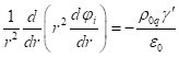
The
inhomogeneous electromagnetic wave equation for the scalar potential inside the
sphere has the standard form:
 . (1)
. (1)
In (1) the Lorentz factor of typical particles is ![]() ,
, ![]() is the average velocity of motion of
an arbitrary particle inside the sphere,
is the average velocity of motion of
an arbitrary particle inside the sphere, ![]() is the speed of light,
is the speed of light, ![]() is the vacuum permittivity,
is the vacuum permittivity, ![]() is the particle’s charge density
in the reference frame associated with the particle, the index
is the particle’s charge density
in the reference frame associated with the particle, the index ![]() distinguishes the internal
potential
distinguishes the internal
potential ![]() from the external potential
from the external potential ![]() , which is generated by the sphere outside its limits. The value
, which is generated by the sphere outside its limits. The value ![]() in (1) represents the effective charge
density. Both the potential
in (1) represents the effective charge
density. Both the potential ![]() and
and ![]() are the functions of the current
radius
are the functions of the current
radius ![]() inside the sphere and they do not depend on the angular variables or
the time due to the stationarity of all the fields. Therefore, in the spherical coordinates, in the Laplacian it is enough to take only the part which depends on the radius:
inside the sphere and they do not depend on the angular variables or
the time due to the stationarity of all the fields. Therefore, in the spherical coordinates, in the Laplacian it is enough to take only the part which depends on the radius:
 .
.
If we make substitution of variables in the form ![]() , then the equation can be rewritten as follows:
, then the equation can be rewritten as follows:
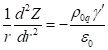 .
.
The dependence of ![]() on the radius was calculated in [1]:
on the radius was calculated in [1]:
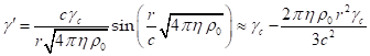 , (2)
, (2)
where ![]() is the Lorentz factor of the
particles in the center of the sphere,
is the Lorentz factor of the
particles in the center of the sphere, ![]() is the acceleration field
coefficient,
is the acceleration field
coefficient, ![]() is the invariant mass density of
the particles.
is the invariant mass density of
the particles.
Substituting (2) into the equation for ![]() , we have:
, we have:
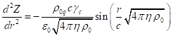 .
.
The general solution of this equation has the form:
 .
.
Since ![]() , and in the center at
, and in the center at ![]() the potential cannot be infinite, the
coefficient
the potential cannot be infinite, the
coefficient ![]() must be equal to zero. Hence, the
potential inside the sphere will equal:
must be equal to zero. Hence, the
potential inside the sphere will equal:
 . (3)
. (3)
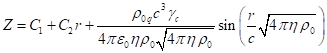
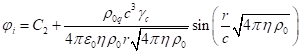
Let us now pass on to calculation of the external
electric potential ![]() of the fixed sphere, filled with
moving charged particles. First, we will find the strength of the external
electric field of the sphere. The Maxwell equations of the electromagnetic
field have the standard form:
of the fixed sphere, filled with
moving charged particles. First, we will find the strength of the external
electric field of the sphere. The Maxwell equations of the electromagnetic
field have the standard form:
![]() ,
,
![]() ,
,
![]() ,
,
![]() . (4)
. (4)
According to (4), the particles moving inside the
sphere at velocities ![]() generate around themselves the
electromagnetic field with the strength
generate around themselves the
electromagnetic field with the strength ![]() and the magnetic field
and the magnetic field ![]() . Let us surround the sphere with the shell of a spherical shape with an
arbitrary radius
. Let us surround the sphere with the shell of a spherical shape with an
arbitrary radius ![]() and integrate the first equation
in (4) over the volume of the shell. We will also apply the Gauss theorem,
replacing the integral of the divergence
and integrate the first equation
in (4) over the volume of the shell. We will also apply the Gauss theorem,
replacing the integral of the divergence ![]() with the integral of the vector
with the integral of the vector ![]() over the surface
over the surface ![]() of the shell. Due to the symmetry
of the sphere at the constant density
of the shell. Due to the symmetry
of the sphere at the constant density ![]() , for the vector
, for the vector ![]() outside the sphere we find the
following:
outside the sphere we find the
following:
![]() . (5)
. (5)
The vector ![]() in (5) denotes the unit normal
vector to the surface of the shell, directed outward. The integration over the
volume
in (5) denotes the unit normal
vector to the surface of the shell, directed outward. The integration over the
volume ![]() of the shell is reduced to
integration over the volume
of the shell is reduced to
integration over the volume ![]() of the sphere, since outside the
sphere
of the sphere, since outside the
sphere ![]() . Substituting here
. Substituting here ![]() from (2) and integrating, we
obtain the magnitude of the field strength outside the
sphere and the field strength itself, directed radially:
from (2) and integrating, we
obtain the magnitude of the field strength outside the
sphere and the field strength itself, directed radially:
 . (6)
. (6)
 .
.
The mass ![]() in (6) is defined as the product
of the mass density
in (6) is defined as the product
of the mass density ![]() by the volume of the sphere. The
supplementary charge
by the volume of the sphere. The
supplementary charge ![]() is equal to the product of the
charge density
is equal to the product of the
charge density ![]() by the volume of the sphere:
by the volume of the sphere: ![]() . However, actually the electric field outside the sphere is defined by
the charge
. However, actually the electric field outside the sphere is defined by
the charge ![]() , which equals according to (5-6):
, which equals according to (5-6):
The relationship between the vectors of the
electromagnetic field and the four-potential is the following:
![]() ,
, ![]() ,
(7)
,
(7)
and where the indices ![]() do not coincide with each other.
do not coincide with each other.
The space components ![]() of the four-potential are the
components of the vector potential
of the four-potential are the
components of the vector potential ![]() , which in this case is equal to zero. Consequently, in (7) the
components
, which in this case is equal to zero. Consequently, in (7) the
components ![]() of the vector
of the vector ![]() are associated only with the time
component
are associated only with the time
component ![]() of the four-potential:
of the four-potential: ![]() . This equality in vector notation is written as follows:
. This equality in vector notation is written as follows: ![]() . Hence, in view of expression (6), for
. Hence, in view of expression (6), for ![]() it follows that:
it follows that:
 .
.
 . (8)
. (8)
At infinity, this potential becomes equal to zero. At
the surface of the sphere potential (8) must coincide with the internal
potential in (3). Let us assume that ![]() and equate the two potentials. This
allows us to determine the coefficient
and equate the two potentials. This
allows us to determine the coefficient ![]() and to specify the internal
potential
and to specify the internal
potential ![]() :
:
![]() ,
,
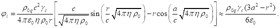
(9)
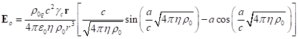
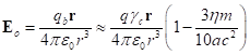
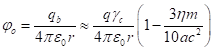
Now we can calculate the electric field strength
inside the sphere. Taking into account the equality of the vector potential ![]() to zero, we have
the following:
to zero, we have
the following:
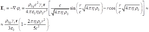
(10)
In (10) we added the following expansion term, which
contained the squared speed of light in the denominator and showed the
difference of the relativistic uniform system from the classical case.
3. The energy of the particles and the field
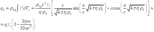
We will first
calculate the contribution into the system’s relativistic energy from the
energy of particles in the electric field, which was defined in [8] as the integral over the volume taken with
respect to the product of the effective charge density inside the sphere ![]() by the internal scalar potential
by the internal scalar potential ![]() .
In view of (2) and (9), we have:
.
In view of (2) and (9), we have:
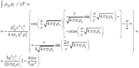 (11)
(11)
Note that the
value of the energy obtained in (11) is twice as large as the electrostatic
energy of the charged particles inside the sphere. We will now calculate the integral over the volume of
the tensor invariant of the electromagnetic field, separately for the field
inside and outside the sphere. The integral of the tensor invariant is
expressed in terms of the electric field strength and the magnetic density:
![]() .
.
This integral is included in this form in the
relativistic energy of the system, where it makes the contribution from the
electromagnetic field [8]. Substituting here (10) and (6), and taking into
account that ![]() ,
we find:
,
we find:
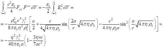
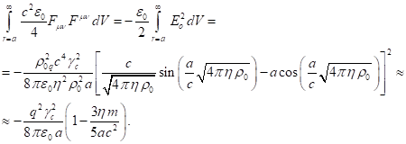
(12)
Conclusions
In [10], in
the framework of the covariant theory of gravitation, a conclusion was made for
the gravitational field that the contribution into the relativistic energy of
the system from the energy of the matter at rest in the gravitational scalar
potential was
twice as large in its absolute value as the
integral of the tensor invariant of the gravitational field, and the same held
true for the electromagnetic field. Would it be different in case of the
relativistic uniform system, where the particles of matter are not motionless,
but are moving with the Lorentz factor (2), which depends on the current radius?
To answer this question, we can sum up the integrals
in (12) taken with respect to the tensor invariant both inside and outside the
sphere, and compare the result with (11). This
gives the
following:
![]()
(13)
Thus, the relation for the energies does not depend on
the type of system uniformity – both in the classical and relativistic cases,
the relation remains the same. It should be noted that due to the random motion
of particles the total magnetic field induction is zero everywhere, and
therefore the sum of the integrals on the left side of (13) is equal in its
absolute value to the electric potential energy of the system.
At first glance, such a coincidence may seem
occasional. Indeed, the contribution into the relativistic energy of the system
from the energy of the particles in the electric field from (11) is twice as
large as the electric potential energy, and at ![]() it is up to a sign equal to the
double value of the integral of the tensor invariant on the left-hand side of
(13). However, it is generally accepted that the electromagnetic field energy
is positive and is calculated by volume integration of the temporary component
it is up to a sign equal to the
double value of the integral of the tensor invariant on the left-hand side of
(13). However, it is generally accepted that the electromagnetic field energy
is positive and is calculated by volume integration of the temporary component ![]() of the stress-energy tensor of
the electromagnetic field. The field energy obtained this way differs by its
sign from the integral of the tensor invariant, which is negative. Hence it
follows that the terms in the relativistic energy of the system, which are
responsible for the energy of the particles in the electromagnetic field and
for the energy of the electromagnetic field itself, differ both from the
electric potential energy and from the field energy, calculated with the help
of the stress-energy tensor.
of the stress-energy tensor of
the electromagnetic field. The field energy obtained this way differs by its
sign from the integral of the tensor invariant, which is negative. Hence it
follows that the terms in the relativistic energy of the system, which are
responsible for the energy of the particles in the electromagnetic field and
for the energy of the electromagnetic field itself, differ both from the
electric potential energy and from the field energy, calculated with the help
of the stress-energy tensor.
Given that the effective charge density inside the
sphere is ![]() , the two variants of estimating the electric potential energy used in
electrostatics can be represented as follows:
, the two variants of estimating the electric potential energy used in
electrostatics can be represented as follows:
![]() .
(14)
.
(14)
The electric potential energy ![]() represents the total contribution
into the relativistic energy of the system made due to the presence of the
electric charges in the system. Thus, in [11] the energy
represents the total contribution
into the relativistic energy of the system made due to the presence of the
electric charges in the system. Thus, in [11] the energy ![]() is calculated using the method of
virtual work by transferring the charges from infinity to the sphere until the
sphere achieves a certain radius. While this work is performed, the charges
acquire energy in the electric potential of the sphere, and the energy of the
field itself increases. Thus, the energy
is calculated using the method of
virtual work by transferring the charges from infinity to the sphere until the
sphere achieves a certain radius. While this work is performed, the charges
acquire energy in the electric potential of the sphere, and the energy of the
field itself increases. Thus, the energy ![]() contains two components – the
energy of the charges in the electric potential and the field energy.
contains two components – the
energy of the charges in the electric potential and the field energy.
Let us now sum up the left-hand sides of equations
(11) and (13) to find the total contribution into the relativistic energy of
the system, arising due to the presence of the electric charges. If we take
into account the right-hand side of (13) and the definition of the electric
potential energy (14), we will again obtain the energy ![]() . This shows that indeed the contribution into the system’s energy is
made by the energy of the charges in the electric potential as well as by the
field energy. However, as mentioned above, these energies coincide neither with
the electric potential energy nor with the field energy, found using the
stress-energy tensor of the electromagnetic field. This arises due to
difference between the covariant approach that takes into account the principle
of least action and the noncovariant approach of the classical electrostatics.
. This shows that indeed the contribution into the system’s energy is
made by the energy of the charges in the electric potential as well as by the
field energy. However, as mentioned above, these energies coincide neither with
the electric potential energy nor with the field energy, found using the
stress-energy tensor of the electromagnetic field. This arises due to
difference between the covariant approach that takes into account the principle
of least action and the noncovariant approach of the classical electrostatics.
Note also that relation (13) can be interpreted as an
example of action of the theorem of equipartition of energy. According to
this theorem, the degrees of freedom, included in the Hamiltonian
quadratically, contribute to the energy of the system two times less than the
degrees of freedom, included in the Hamiltonian linearly [12]. The electric
field strength is included in the tensor invariant quadratically and the
electric field potential is included in relativistic energy linearly. As a
result, according to (13), the field strength and the field potential can be
considered separate and independent degrees of freedom of the electromagnetic
field, which are equally necessary for description of the processes in the
field.
References
1.
Fedosin S.G. Relativistic Energy and Mass in the Weak Field Limit. Jordan Journal of Physics. Vol. 8, No. 1, pp. 1-16 (2015).
2.
Fedosin S.G. The Integral Energy-Momentum 4-Vector and Analysis of
4/3 Problem Based on the Pressure Field and Acceleration Field. American Journal of Modern Physics.
Vol. 3, No. 4, pp.
152-167 (2014). http://dx.doi.org/10.11648/j.ajmp.20140304.12.
3.
Fedosin S.G. Estimation of the physical
parameters of planets and stars in the gravitational equilibrium model.
Canadian Journal of Physics, Vol. 94, No.
4, pp. 370-379 (2016). http://dx.doi.org/10.1139/cjp-2015-0593.
4.
Fedosin S.G. The radius of the proton in the self-consistent model. Hadronic Journal,
Vol. 35, No. 4, pp. 349-363 (2012).
5.
Kelly J. J. Nucleon Charge and Magnetization Densities, arXiv:hep-ph/0111251.
6.
Ulugbek Yakhshiev and Hyun-Chul Kim. Transverse charge densities in the nucleon in
nuclear matter. Physics Letters B, Vol. 726, Issues 1–3, pp. 375-381 (2013). http://dx.doi.org/10.1016/j.physletb.2013.08.004.
7.
Fedosin S.G. The Procedure of Finding the Stress-Energy Tensor and
Equations of Vector Field of Any Form.
Advanced Studies in Theoretical Physics, Vol. 8, No. 18, pp. 771-779 (2014). http://dx.doi.org/10.12988/astp.2014.47101.
8.
Fedosin S.G. About the cosmological constant, acceleration field,
pressure field and energy. Jordan Journal of Physics, Vol. 9, No. 1, pp. 1-30 (2016).
9.
Fedosin S.G. The virial theorem and the
kinetic energy of particles of a macroscopic system in the general field
concept. Continuum
Mechanics and Thermodynamics, Vol. 29, Issue 2, pp. 361-371 (2016). https://dx.doi.org/10.1007/s00161-016-0536-8.
10.
Fedosin S.G. The Hamiltonian in Covariant Theory of Gravitation. Advances in Natural Science, Vol. 5, No. 4, pp. 55-75
(2012). http://dx.doi.org/10.3968%2Fj.ans.1715787020120504.2023.
11.
Feynman R, Leighton R, and Sands M. The Feynman
Lectures on Physics. Volume 2. Addison Wesley, 1964.
12.
Huang, K. (1987). Statistical Mechanics (2nd ed.).
John Wiley and Sons. pp. 136–138.
Source: http://sergf.ru/elpen.htm