На русском языке

Jordan Journal of Physics. Vol. 9 (No. 1), pp. 1-30, (2016). http://journals.yu.edu.jo/jjp/Vol9No1Contents2016.html

About the cosmological constant, acceleration field, pressure field and energy

Sergey G. Fedosin

PO box 614088, Sviazeva str. 22-79, Perm, Russia

E-mail: intelli@list.ru

Based on the condition of relativistic energy uniqueness the calibration of the cosmological constant was performed. This allowed us to obtain the corresponding equation for the metric, to determine the generalized momentum, the relativistic energy, momentum and the mass of the system, as well as the expressions for the kinetic and potential energies. The scalar curvature at an arbitrary point of the system equaled zero, if the substance is absent at this point; the presence of a gravitational or electromagnetic field is enough for the space-time curvature. Four-potentials of the acceleration field and pressure field, as well as tensor invariants determining the energy density of these fields, were introduced into the Lagrangian in order to describe the system’s motion more precisely. The structure of the Lagrangian used is completely symmetrical in form with respect to the 4-potentials of gravitational and electromagnetic fields and acceleration and pressure fields. The stress-energy tensors of the gravitational, acceleration and pressure fields are obtained in explicit form, each of them can be expressed through the corresponding field vector and additional solenoidal vector. A description of the equations of acceleration and pressure fields is provided.

Keywords: cosmological constant; 4-momentum; acceleration field; pressure field; covariant theory of gravitation.

PACS: 04.20.Fy, 04.40.-b, 11.10.Ef

1. Introduction

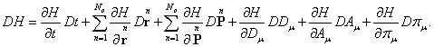
The most popular application of the cosmological constant in the general theory of relativity (GTR) is that this quantity represents the manifestation of the vacuum energy [1-2]. There is another approach to the cosmological constant interpretation, according to which this quantity represents the energy possessed by any solitary particle in the absence of external fields. In this case, including into the Lagrangian seems quite appropriate since the Lagrangian contains such energy components, which should fully describe the properties of any system consisting of particles and fields.

Earlier in [3-4] we used such calibration of the cosmological constant, which allowed us to maximally simplify the equation for the metric. The disadvantage of this approach was that the relativistic energy of the system could not be determined uniquely, since the expression for the energy included the scalar curvature. In this paper we use another universal calibration of the cosmological constant, which is suitable for any particle and system of particles and fields. As a result, the energy is independent of both the scalar curvature and the cosmological constant.

In GTR the gravitational field as a separate object is not included in the Lagrangian, and the role of a field is played by the metric itself. A known problem arising from such an approach is that in GTR there is no stress-energy tensor of the gravitational field.

In contrast, in the covariant theory of gravitation the Lagrangian is used containing the term with the energy of the particles in the gravitational field and the term with the energy of the gravitational field as such. Thus, the gravitational field is included in the Lagrangian in the same way as the electromagnetic field. In this case, the metric of the curved spacetime is used to specify the equations of motion as compared to the case of such a weak field, the limit of which is the special theory of relativity. In the weak field limit a simplified metric is used, which almost does not depend on the coordinates and time. This is enough in many cases, for example, in case of describing the motion of planets. However, generally, in case of strong fields and for studying the subtle effects the use of metric becomes necessary.

We will note that the term with the particle energy in the Lagrangian can be written in different ways. In [5-6] this term contains the invariant , where is the mass density in the co-moving reference frame, is 4-velocity. The corresponding quantity in [7] has the form . In [3] and [8] instead of it the product is used, where is mass 4-current. In this paper we have chosen another form of the mentioned invariant – in the form . The reason for this choice is the fact that we consider the mass 4-current to be the fullest representative of the properties of substance particles containing both the mass density and the 4-velocity. The mass 4-current can be considered as the 4-potential of the matter field. All the other 4-vectors in the Lagrangian are 4-potentials of the respective fields and are written with covariant indices. With the help of these 4-potentials tensor invariants are calculated which characterize the energy of the respective field in the Lagrangian.

2. Action and its variations in the principle of least action

2.1. The action function

We use the following expression as the action function for continuously distributed matter in the gravitational and electromagnetic fields in an arbitrary frame of reference:

(1)

where – the Lagrange function or Lagrangian,

– the differential of the coordinate time of the used reference frame,

– a coefficient to be determined,

– the scalar curvature,

– the cosmological constant,

– the 4-vector of gravitational (mass) current,

– the mass density in the reference frame associated with the particle,

– the 4-velocity of a point particle, – 4-displacement, – interval,

– the speed of light as a measure of the propagation velocity of electromagnetic and gravitational interactions,

– the 4-potential of the gravitational field, described by the scalar potential and the vector potential of this field,

– the gravitational constant,

– the gravitational tensor (the tensor of gravitational field strengths),

– definition of the gravitational tensor with contravariant indices by means of the metric tensor ,

– the 4-potential of the electromagnetic field, which is set by the scalar potential and the vector potential of this field,

– the 4-vector of the electromagnetic (charge) current,

– the charge density in the reference frame associated with the particle,

– the vacuum permittivity,

– the electromagnetic tensor (the tensor of electromagnetic field strengths),

– the 4-velocity with a covariant index, expressed through the metric tensor and the 4-velocity with a contravariant index; it is convenient to consider the covariant 4-velocity locally averaged over the particle system as the 4-potential of the acceleration field , where and denote the scalar and vector potentials, respectively,

– the acceleration tensor calculated through the derivatives of the four-potential of the acceleration field,

– a function of coordinates and time,

– the 4-potential of the pressure field, consisting of the scalar potential and the vector potential , is the pressure in the reference frame associated with the particle, the relation specifies the equation of the substance state,

– the tensor of the pressure field,

– a function of coordinates and time,

– the invariant 4-volume, expressed through the differential of the time coordinate , through the product of differentials of the spatial coordinates and through the square root of the determinant of the metric tensor, taken with a negative sign.

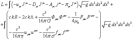
Action function (1) consists of almost the same terms as those which were considered in [3]. The difference is that now we replace the term with the energy density of particles with four terms located at the end of (1). It is natural to assume that each term is included in (1) relatively independently of the other terms, describing the state of the system in one way or another. The value of the 4-potential of the set of matter units or point particles of the system defines the 4-field of the system’s velocities, and the product in (1) can be regarded as the energy of interaction of the mass current with the field of velocities.

Similarly, is the 4-potential of the gravitational field, and the product defines the energy of interaction of the mass current with the gravitational field. The electromagnetic field is specified by the 4-potential , the source of the field is the electromagnetic current , and the product of these quantities is the density of the energy of interaction of a moving charged substance unit with the electromagnetic field. The invariant of the gravitational field in the form of the tensor product is associated with the gravitational field energy and cannot be equal to zero even outside bodies. The same holds for the electromagnetic field invariant . This follows from the properties of long-range action of the specified fields. As for the field of velocities , the field should be used to describe the motion of the substance particles. Accordingly, the field of accelerations in the form of the tensor and the energy of this field associated with the invariant refer to the accelerated motion of particles and are calculated for those spatial points within the system’s volume where the substance is located.

The last two terms in (1) are associated with the pressure in the substance, and the product characterizes the interaction of the pressure field with the mass 4-current, and the invariant is part of the stress-energy tensor of the pressure field.

We will also note the difference of 4-currents and – all particles of the system make contribution to the mass current , and only charged particles make contribution to the electromagnetic current . This results in difference of the fields’ influence – the gravitational field influences any particles and the electromagnetic field influences only the charged particles or the substance, in which by the field can sufficiently divide with its influence the charges of opposite signs from each other. The field of velocities , as well as the mass current , are associated with all the particles of the system. Therefore, the product describes that part of the particles’ energy, which stays if we somehow "turn off " in the system under consideration all the macroscopic gravitational and electromagnetic fields and remove the pressure, without changing the field of velocities or the mass current .

2. 2. Variations of the action function

We will vary the action function in (1) term by term, then the total variation will be the sum of variations of individual terms. In total there are 9 terms inside the integral in (1). If we consider the quantity a constant (a cosmological constant), then according to [7-9] the variation of the first term in the action function (1) is equal to:

, (2)

where is the Ricci tensor,

is the variation of the metric tensor.

According to [3] the variations of terms 2 and 3 in the action function are as follows:

, (3)

, (4)

where is the variation of coordinates, which results in the variation of the mass 4-current and in the variation of the electromagnetic 4-current ,

is the variation of the 4-potential of the gravitational field,

and denotes the stress-energy tensor of the gravitational field:

. (5)

Variations of terms 4 and 5 in the action function according to [6-7], [10] are as follows:

, (6)

, (7)

where is the variation of the 4-potential of the electromagnetic field,

and denotes the stress-energy tensor of the electromagnetic field:

. (8)

Variations of the other terms in the action function (1) are defined in Appendices A-D and have the following form:

, (9)

, (10)

where is the variation of the 4-potential of the acceleration field,

and denotes the stress-energy tensor of the field of accelerations:

. (11)

(12)

, (13)

where the stress-energy tensor of the pressure field:

. (14)

In variation (10) in order to simplify the special case is considered, when is a constant, which does not vary by definition. According to its meaning depends on the parameters of the system under consideration, and therefore can have different values. The same should be said about .

3. The motion equations of the field, particles and metric

According to the principle of least action, we should sum up all the variations of the individual terms of the action function and equate the result to zero. The sum of variations (2), (3), (4), (6), (7), (9), (10), (12) and (13) gives the total variation of the action function:

. (15)

3.1. The field equations

When the system moves in spacetime, the variations , , , , and do not vanish, since it is supposed that it can occur only at the beginning and the end of the process, when the conditions of motion are precisely fixed. Consequently, the sum of the terms, which is located before these variations, should vanish. For example, the variation occurs only in according to (6 ) and in from (7), then from (15) it follows:

.

From this we obtain the equation of the electromagnetic field with the field sources:

or , (16)

where is the vacuum permeability.

The second equation of the electromagnetic field follows from the definition of the electromagnetic tensor in terms of the electromagnetic 4-potential and from the antisymmetry properties of this tensor:

or , (17)

where is a Levi-Civita symbol or a completely antisymmetric unit tensor.

The variation is present only in (3) and (4), so that according to (15) we should obtain:

.

The equation of gravitational field with the field sources follows from this:

or . (18)

If we take into account the definition of the gravitational tensor: , and take the covariant derivative of this tensor with subsequent cyclic interchange of the indices, the following equations are solved identically:

or . (19)

Equation (19) without the sources and equation (18) with the sources define a complete set of gravitational field equations in the covariant theory of gravitation.

Consider now the rule for the difference of the second covariant derivatives with respect to the covariant derivative of the electromagnetic 4-potential :

With the rule in mind, the applying of the covariant derivative to (16) and (18) gives the following:

.

.

This shows that field tensors and lead to the divergence of the corresponding 4-currents in a curved space-time. Mixed curvature tensor and Ricci tensor vanish only in Minkowski space. In this case, the covariant derivatives become the partial derivatives and the continuity equation for the gravitational and electromagnetic 4-currents in the special theory of relativity are obtained:

, . (20)

We will note that in order to simplify the equations for the 4-potential of fields we can use expressions which are called gauge conditions:

, . (21)

3.2. The acceleration field equations

The variation of 4-potential is included in (9) and (10), therefore according to (15) we should obtain:

.

, or . (22)

If we compare (18) and (22), it turns out that the presence of the 4-vector of mass current not only leads to occurrence of space-time gradient of the gravitational field in the system under consideration, but is generally accompanied by changes in time or by 4-velocity gradients of the particles that constitute this system. Besides the covariant 4-velocities of the whole set of particles forms the velocity field , the derivatives of which define the acceleration field and are described by the tensor . As an example of a system, where it can be clearly observed, we can take a rotating partially-charged collapsing gas-dust cloud, held by gravity. An ordered acceleration field occurs in the cloud due to the rotational acceleration and contains the centripetal and tangential acceleration.

Due to its definition in the form of a 4-rotor of , the following relations hold for acceleration tensor :

or . (23)

As we can see, the structure of equations (22) and (23) for the acceleration field is similar to the structure of equations for the strengths of gravitational and electromagnetic fields.

In the local geodetic reference frame the derivatives of the metric tensor and the curvature tensor become equal to zero, the covariant derivative becomes a partial derivative and the equations take the simplest form. We will go over to this reference frame and apply the derivative to (23) and make substitution for the first and third terms using (22):

.

If we apply definition to 4-d’Alembertian , where is the d'Alembert operator, it will give:

.

Comparing with the previous expression, we find the wave equation for the 4-potential :

.

On the other hand, after lowering of the acceleration tensor indices we have from (22):

.

Comparing this equation with equation for leads to the expression:

,

where is some constant.

In an arbitrary reference frame we should specify the obtained expressions, since in contrast to permutations of partial derivatives, in case of permutation of the covariant derivatives from the sequence to the sequence some additional terms appear. In particular, if we use the relation:

, (24)

then after substituting the expression in (22), the wave equation can be written as follows:

. (25)

In the curved space operator acts differently on scalars, 4-vectors and 4-tensors, and usually it contains the Ricci tensor. Due to condition (24), the Ricci tensor is absent in (25), but the terms with the Christoffel symbols remain.

Equation (24) is a gauge condition for the 4-potential , which is similar by its meaning to gauge conditions (21) for the electromagnetic and gravitational 4-potentials. Both (24) and (25) will hold on condition that .

In Appendix E it will be shown that the acceleration tensor includes the vector components and , based on which, according to (E6), we can build a 4-vector of particles’ acceleration.

3.3. The pressure field equations

To obtain the pressure field equations we need to choose in (15) those terms which contain the variation . This variation is present in (12) and (13), which gives the following:

.

or . (26)

It follows from (26) that the mass 4-current generates the pressure field in bodies, which can be described by the pressure tensor . The same relations hold for this tensor as for the tensors of other fields:

or . (27)

The wave equation for the 4-potential of the pressure field follows from (26) and (27):

. (28)

Equations (26) and (28) will be consistent at the same time if there is gauge condition of the pressure 4-potential:

, (29)

where is some constant. As a rule, these constants are chosen to be equal to zero.

The properties of the pressure field are described in Appendix F, where it is shown that the pressure tensor contains two vector components and , which determine the energy and the pressure force, as well as the pressure energy flux.

3.4. The equations of motion of particles

The variation that leads to the equations of motion of the particles is present in (3), (6), (9) and (12). For this variation it follows from (15):

,

.

The left side of the equation can be transformed, considering the expression for the 4-vector of mass current density and the definition of the acceleration tensor :

. (30)

We used the relation , which follows from the equation , and the operator of proper-time-derivative as operator of the derivative with respect to the proper time , where is a symbol of 4-differential in curved spacetime, is the proper time [11]. Taking into account (30) the equation of motion takes the form:

. (31)

We will note that the equations of field motion (16) – (19), of the acceleration field (22) and (23), of the pressure field (26) and (27) and the equation of the particles’ motion (31) are differential equations, which are valid at any point volume of spacetime in the system under consideration. In particular, if the mass density in some point volume is zero, then all the terms in (31) will be zero.

The quantity in the left side of (31) is the 4-acceleration of a point particle, while the proper time differential is associated with the interval by relation: and the relation holds: . The first two terms in the right side of (31) are the densities of the gravitational and electromagnetic 4-forces, respectively. It can be shown (see for example [3], [12]) that for 4-forces, exerted by the field on the particle, there are alternative expressions in terms of the stress-energy tensors (5) and (8):

, . (32)

Similarly, the left side of (31) with regard to (30) is expressed in terms of stress-energy tensor of the acceleration field (11):

. (33)

To prove (33) we should expand the tensor with the help of definition (11), apply the covariant derivative to the tensor products and then use equations (22) and (23). Equation (33) shows that the 4-acceleration of the particle can be described by either the acceleration tensor or the tensor .

For the pressure field we can write the same as for other fields:

. (34)

In (34) the pressure 4-force is associated with the covariant derivative of the stress-energy tensor of the pressure field.

From (31) – (34) it follows:

or . (35)

In Minkowski space , where is present, 4-differetials become ordinary differentials , ,

and the motion equation (31) falls into the scalar and vector equations, while the vector equation contains the total gravitational force with regard to the torsion field, the electromagnetic Lorentz force and the pressure force:

, (36)

, (37)

where is the velocity of a point particle, is the gravitational field strength, is the charge density, is the electric field strength, is the pressure field strength, is the torsion field vector, is the magnetic field induction, is the solenoidal vector of the pressure field.

If during the time the density does not change, it can be put under the derivative’s sign. Then in the left side of (36) the quantity appears, where is the relativistic energy density. Similarly, in the left side of (37) the quantity appears, where is the mass 3-current density.

3.5. The equations for the metric

Let us consider action variations (2), (3), (4), (6), (7), (9), (10), (12) and (13), which contain the variation . The sum of all the terms in (15) with the variation must be zero:

.

(38)

The equation for the metric (38) allows us to determine the metric tensor by the known quantities characterizing the substance and field. If we take the covariant derivative in this equation, the left side of the equation vanishes on condition , and taking into account (35) we obtain the following:

,

, (39)

where is a function of time and coordinates and the scalar invariant with respect to coordinate transformations.

If we expand the scalar products of vectors using the expressions:

, , (40)

.

then (39) can be written as:

. (41)

If the system’s substance and charges are divided to small pieces and scattered to infinity, then there the external field potentials become equal to zero, since interparticle interaction tends to zero, and at we obtain the following:

. (42)

Consequently, is associated with the particle’s proper scalar potentials and , the mass density and the pressure in the particle located at infinity. Expression (41) can be considered as the differential law of conservation of mass-energy: the greater the velocity of a point particle is, and the greater the gravitational field potentials and , the electromagnetic field potentials and , the pressure field potentials and are, the more the mass density differs from its value at infinity. For example, if a point particle falls into the gravitational field with the potential , then the change in the particle’s energy is described by the term . According to (41), such energy change can be compensated by the change in the rest energy of the particle due to the change . Since the gravitational field potential is always negative, then the mass density and the pressure inside the point particle should increase due to the field potential.

This is possible, if we remember that the whole procedure of deriving the motion equations of particles, field and metric from the principle of least action is based on the fact that the mass and charge of the substance unit at varying of the coordinates remain constant, despite of the change in the charge density, substance density and its volume [7]. If the mass of a simple system in the form of a point particle and the fields associated with it is proportional to , then according to (41) the mass of such a system remains unchanged, despite of the change in the fields, mass density and pressure . Conservation of the mass-energy of each particle with regard to the mass-energy of the fields leads to conservation of the mass-energy of an arbitrary system including a multitude of particles and the fields surrounding them. We will remind that this article refers to the continuously distributed matter, so that each point particle or a unit of this matter may have its own mass density and its value .

We will now return to (38) and take the contraction of tensors by means of multiplying the equation by , taking into account the relation , and then dividing all by 2:

. (43)

where is the scalar curvature, and it was taken into account that the contractions of tensors , , and are equal to zero.

In case if the cosmological constant were known, based on (43) we could find the scalar curvature .

In order to simplify the equation (38) in [3] and [4] we introduced the gauge for , at which the following equation would hold, if we additionally take into account the term with the pressure :

. (44)

In the gauge (44) the equation for the metric (38) takes the following form, provided that , where is a constant of order of unity:

. (45)

We will note that if from the right side of (45) we exclude the stress-energy tensor of the gravitational field , replace the tensor with the stress-energy tensor of the substance in the form , and also neglect the tensor , then at we will obtain a typical equation for the metric used in the general theory of relativity:

. (46)

The equation for the metric (38) and the expression (39) must hold in the covariant theory of gravitation, provided that . If in (39) we remove the term , then we will obtain an expression suitable for use in the general theory of relativity. In this case, given that , instead of (39) we obtain the following:

. (47)

If in (47) we equate the term with the energy of particles in the electromagnetic field (in the case when the field is zero) to zero, then the sum of the rest energy density and the pressure energy of each uncharged point particle must be unchanged. It follows that the pressure change must be accompanied by a change in the mass density. If the system contains the electromagnetic field with the 4-potential acting on the 4-currents generating them, then in the general case there must be inverse correlation of the rest energy, pressure energy and the energy of charges in the electromagnetic field.

Indeed, in the general theory of relativity the mass density determines the rest energy density and spacetime metric, which represents the gravitational field. In (47) the energy of charges in the electromagnetic field is specified by the term , and the mass density and hence the metric are associated with this energy at a constant . On the other hand, the metric is obtained from (46). Therefore, the occurrence of the electromagnetic field influences the metric in two relations — in (47) the mass density and the corresponding metric change, as well as in the equation for the metric (46) the stress-energy tensor of the substance changes, while the stress-energy tensor of the electromagnetic field also makes contribution to the metric.

A well-known paradox of general theory of relativity is associated with all of this — the electromagnetic field influences the density, the mass of the bodies as the source of gravitation, and the metric, while the gravitational field itself (i.e. metric) does not influence the electrical charges of the bodies, which are the sources of the electromagnetic field. Thus the gravitational and electromagnetic fields are unequal relative to each other, despite the similarity of field equations and the same character of long-range action. Above we pointed out at the fact that the mass 4-current leads to the gravitational field gradients, and the addition of the charge to this mass current generates additional electromagnetic (charge) 4-current and the corresponding electromagnetic field gradients, depending on the sign of the charge. From this we can see that the gravitational field looks like a fundamental, basic and indestructible field and the electromagnetic field manifests as some superstructure and the result of the charge separation in the initially neutral substance.

If we consider (44) to be valid, then from comparison with (39) we see that the equation must be satisfied. Thus, when is considered as a cosmological constant, we can use it to achieve simplification of the equation for the metric (38) and bring it to the form of (45). At the same time the relation (39) is symmetrical with respect to the contribution of the gravitational and electromagnetic fields to the density, in spite of the difference in fields. We will remind that in the equation of motion (31) both fields also make symmetrical contributions to the 4-acceleration of a point charge.

Although the gauge for in the form of (44) seems the simplest and simplifies some of the equations, in Section 7 the necessity and convenience of another gauge will be shown.

4. Hamiltonian

In this and the next sections we rely on the standard approach of analytical mechanics. As the coordinates it is convenient to choose a set of Cartesian coordinates: , , , .

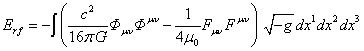
Let us consider action (1) and express the Lagrangian from it:

(48)

The integration in (48) is carried out over the infinite three-dimensional volume of space and over all the material particles of the system. We assume that the scalar curvature depends on the metric tensor, and the metric tensor , the field tensors , , , , the density , the charge density and the pressure are functions of the coordinates and do not depend on the particle velocities. Then the Lagrangian in its general form (48) depends on the coordinates, as well as on the 4-potential of pressure and 4-potentials of the gravitational and electromagnetic fields and .

We will divide the first integral in the Lagrangian (48) to the sum of particular integrals, each of which describes the state of one of the set of the system’s particles. We will take into account also that the Lagrangian depends on the three-dimensional velocities of the particles , where specifies the particle’s number, while the velocity of any particle is part of only one corresponding particular integral. If we denote by the second integral in (48), which is associated with the energies of fields inside and outside the fixed physical system and is independent of the particles’ velocities, then we can write for the Lagrangian:

,

where is a particular Lagrangian of an arbitrary particle.

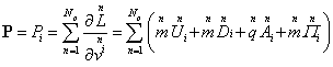
We will introduce now the Hamiltonian of the system as a function of generalized three-dimensional momenta of the particles: . Under the system’s generalized momentum we mean the sum of the generalized momenta of the whole set of particles:

.

To find the Hamiltonian we will apply the Legendre transformations to the system of particles:

, (49)

provided that

. (50)

The equality in (50) gives the definition of the generalized momentum , and we can see that the generalized momentum of an arbitrary particle equals . On the other hand, the equations allow us to express the velocity of an arbitrary particle through its generalized momentum . Then we can substitute these velocities in (49) and determine only through .

In order to find in (50), in each particular Lagrangian we should express and in terms of the velocity and interval :

, , (51)

while and we introduce the notation , where the four-dimensional quantity is not a real 4-vector. With regard to the definition of the 4-potential of the acceleration field , for each particle we obtain:

. (52)

In (48) the unit of volume of the system in any particular integral can be expressed in terms of the unit of volume in the reference frame associated with the particle in the following way:

. (53)

From this formula in the weak-field limit in Minkowski space, when , it follows that the volume of a moving particle is decreased in comparison with the volume of a particle at rest. Given that , where is the proper time in the reference frame of the particle, the equality of 4-volumes in different reference frames follows from (53):

.

This equation reflects the fact that the 4-volume is a 4-invariant.

Under the above conditions (40), (51), (52) and (53) can be written for the Lagrangian (48) as follows:

(54)

as well as after partial volume integration:

(55)

where is the mass of an arbitrary particle, is the particle’s charge. In (55) the scalar and vector field potentials are averaged over the particle’s volume, that means they are the effective potentials at the location of the particle.

In operations with 3-vectors it is convenient to write vectors in the form of components or projections on the spatial axes of the coordinate system using, for example, instead of the velocity the quantity , where . Then , , and the velocity derivative can be represented as: . For the gravitational vector potential in particular we obtain: .

With this in mind, from (55) and (50) we find:

, . (56)

Based on this, we find for the sums of the scalar products of 3-vectors by summing over the index :

. (57)

From (49) taking into account (55) and (57) we have:

(58)

In (58) the Hamiltonian contains the scalar curvature and the cosmological constant . As it will be shown in Section 6 about the energy, this Hamiltonian represents the relativistic energy of the system. To make the picture complete we could also express the quantity in (58) through the generalized momentum . We have described this procedure in [4].

For continuously distributed substance the masses and charges of the particles in (58) can be expressed through the corresponding integrals: , . Also taking into account (53), in which we can substitute the expression , where denotes the time component of the 4-velocity of an arbitrary particle, from (58) we find:

(59)

If in (58) we express the masses and charges of the particles through the mass density and the charge density from the standpoint of the arbitrary reference frame , then (58) can be represented as follows:

(60)

We obtained the Hamiltonian in an arbitrary reference frame , while in (59) the densities in reference frames associated with the particles are used and in (60) such particle densities are used, as they seem to be in .

5. Hamilton’s equations

Assuming that the Hamiltonian depends on the generalized 3-momenta of particles : and the Lagrangian depends on 3-velocity of particles : , where is a three-dimensional radius-vector of the particle with the number , we will take differentials of and , as well as the differentials of both sides of equation (49):

(61)

(62)

. (63)

Substituting (61) and (62) into (63), we find:

, , , ,

, , . (64)

The last equation in (64) leads to (50) and gives the expression (56) for the generalized momentum of an arbitrary particle of the system in an explicit form.

We will now apply the principle of least action to the Lagrangian in the form , equating the action variation to zero, when the particle moves from the time point to the time point .

(65)

In (65) it was assumed that the time variation is equal to zero: . Partial derivatives with variations , and lead to field equations (16), (18) and (26). If we take into account the definition of velocity in the second term in the integral (65): , then the integral for this term is taken by parts. Then for the first and second terms in the integral (65) we have the following:

. (66)

When varying the action, the variations are equal to zero only at the beginning and at the end of the motion, that is when and . Therefore, for vanishing of the variation it is necessary that the quantity in brackets inside the integral (66) would be equal to zero. This leads to the well-known Lagrange equations of motion:

. (67)

According to (64) , as well as . Let us substitute this in (67):

. (68)

Equation (68) together with equation from (64)

represent the standard Hamiltonian equations describing the motion of an arbitrary particle of the system in the gravitational and electromagnetic fields and in the pressure field. According to (68), the rate of change of the generalized momentum of the particle by the coordinate time is equal to the generalized force, which is found as the gradient with respect to the particle’s coordinates of the relativistic energy of the system taken with the opposite sign. These equations are widely used not only in the general theory of relativity, but also in other areas of theoretical physics. We have checked these equations in [4] in the framework of the covariant theory of gravitation by direct substitution of the Hamiltonian.

6. The system’s energy

We will consider a closed system which is in the state of some stationary motion. An example would be a charged ball rotating around its center of mass, which forms the system under consideration together with its gravitational and electromagnetic fields and the internal pressure. In such a system the energy should be conserved as a consequence of lack of energy losses to the environment and taking into account the homogeneity of time, i.e. the equivalence of the time points for the system’s state.

The system’s Lagrangian, taking into account the fields’ energy, has the form of (55). Due to the stationary motion we can assume that within the system’s volume the metric tensor , the scalar curvature , the 4-potentials of the field , and of the pressure do not depend on time. 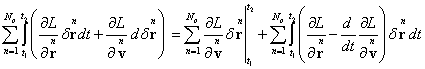But since any point particle moves with the ball, then its location and velocity are changed, being defined by the radius vector and velocity , respectively. We may assume that the Lagrangian of the system does not depend explicitly on time and is a function of the form: . Now we will take the time derivative of the Lagrangian, as it is done for example in [13], only not for one but for a set of particles, and will apply (67):

.

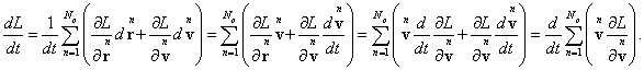
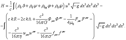
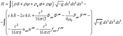
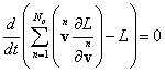
The quantity in the brackets is not time-dependent and is constant. This gives the definition of relativistic energy as a conserved quantity for a closed system at stationary motion:

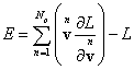. (69)

With regard to (64) and (49), we find the following:

. (70)

It turns out that the relativistic energy can be expressed in a covariant form, since according to (70) the formula for the energy coincides with the formula for the Hamiltonian in (49).

To calculate the relativistic energy of the system with the substance, which is continuously distributed over the volume, it is convenient to pass from the mass and charge of the particle to the corresponding densities inside the particle. According to (59) we obtain:

(71)

Using expression (71) we can find the invariant energy of the system, for which we should use the frame of reference of the center of mass and calculate the integral. In addition, at a known velocity of the center of mass of the system in an arbitrary reference frame we can calculate the momentum of the system in . This can be clarified as follows. We will define the invariant mass of the system taking into account the mass-energy of the fields using the relation: , where is the speed of light as a measure of the velocity of propagation of electromagnetic and gravitational interactions. If the 4-displacement in has the form: , then for the 4-velocity of the system in we can write: . The 4-vector defines the 4-momentum, which contains the relativistic energy and relativistic momentum . This gives the formula for determining the momentum through the energy: , and, correspondingly, for the 4-momentum: .

In the reference frame , in which the system is at rest , , , and then , and also , that is in the 4-momentum in the reference frame only the time component is nonzero.

If we multiply the 4-momentum by the speed of light, we will obtain the 4-vector of the form , the time component of which is the relativistic energy, equal in value to the Hamiltonian. Thus we find the 4-vector, which in [4] was called the Hamiltonian 4-vector.

7. The cosmological constant gauge and the resulting consequences

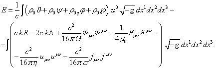
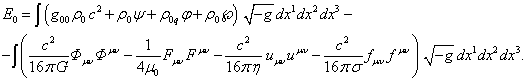
We will make transformations and substitute (43) and (39) in (71):

(72)

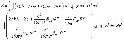
If we choose the condition for the cosmological constant in the form:

, (73)

then the relativistic energy (72) is uniquely defined, since the dependence on the constants and disappears:

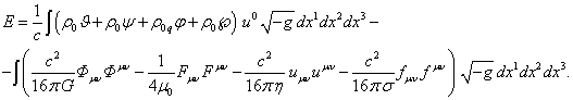(74)

We will remind that the quantities and can have their own values for each particle of matter. But on condition of (73) the expression for the relativistic energy (74) becomes universal for any particle in an arbitrary system of particles and their fields.

From (73) and (39) the equation follows:

. (75)

In order to estimate the value of the cosmological constant , it is convenient to divide all of the system’s substance into small pieces, scatter them apart to infinity and leave there motionless. Then the vector potentials of the fields and pressure become equal to zero and the relation remains: . It follows that , just like in ( 42), is associated with the rest energy, with the pressure energy and with the proper energy of the fields of the system under consideration.

If in some volume there are no particles and the mass density and the charge density are zero, then in this volume there must remain the relativistic energy of the external fields:

. (76)

Based on (74) we can express the energy of a small body at rest. For simplicity we will assume that the body does not rotate as a whole and there is no motion of the substance and charges inside of it (an ideal solid body without the intrinsic magnetic field and the torsion field). Under such conditions the coordinate time of the system becomes approximately equal to the proper time of the body: . Since the interval , then we obtain: . Since there are no spatial motion in any part of the body, we can write:

, .

With this in mind we obtain from (74):

(77)

In the weak field limit in (77) we can use , . The tensor product in the absence of substance motion inside the ideal solid body vanishes. Using (F5) and (F6) we can write:

, , .

Besides in [4] it was found that in the weak field for a motionless body in the form of a ball with uniform density of mass and charge the following relations hold for the body’s proper fields:

, ,

,

. (78)

According to (78) the potential energy of the ball’s substance in the proper gravitational field which is associated with the scalar potential is twice greater than the potential energy associated with the field strength . The same is true for the electromagnetic field with the potential and the strength both in the case of uniform arrangement of charges in the ball’s volume and in case of their location on the surface only. Substituting (78) into (77) in the framework of the special theory of relativity gives the invariant energy of the system in the form of a fixed solid spherical body with uniform density of mass and charge, taking into account the energy of their proper potential fields:

(79)

This calculation is apparently not complete since in reality inside any body there are particles, which cannot be as motionless as the body itself is. Therefore in (79), in addition to the pressure and its gradient within the body it is necessary to add the kinetic energy of motion of all the particles which constitute the body.

7.1. The metric

Substituting (75) and (39) into (43), we find the expression for the scalar curvature :

, (80)

while , where is a constant of the order of unity.

As it can be seen, the scalar curvature is zero in the whole space outside the body. The equation does not mean however, that the spacetime is flat as in the special theory of relativity, since the curvature of spacetime is determined by the components of the Riemann curvature tensor.

We will now substitute (75) into the equation for the metric (38):

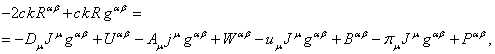(81)

that also can be written using (39) as follows:

. (82)

If we take the covariant derivative of (82), the left side of the equation vanishes due to the property of the Einstein tensor located there. The right side, with regard to the equation of motion (35) and provided that the metric tensor in covariant differentiation behaves as a constant and is a constant, vanishes too.

In (81) we can use (80) to replace the scalar curvature:

(83)

If we sum up (81) and (83) and divide the result by 2 , we will obtain the following equation for the metric:

, (84)

while with regard to (80) , according to (35) , and as the property of the Einstein tensor.

In empty space according to (84) the curvature tensor depends only on the stress-energy tensors of the gravitational and electromagnetic fields and , so these fields change the curvature of spacetime outside the bodies. We will note that in equation (84) the cosmological constant and the tensor product of the type are missing. This fact makes determination of the metric tensor components much easier.

If we compare (84) with the Einstein equation (46), then two major differences will be found out — in the right side of (84 ) stress-energy tensors , and are present, and in addition the coefficient in front of the scalar curvature is two times less than in (46).

8. Компоненты энергии

In Newtonian mechanics the relations for the Lagrangian and the total energy are known: , , where denotes the kinetic energy, which depends only on the velocity, and denotes the potential energy of the system, depending both on the coordinates and the velocity. In relativistic physics instead of individual scalar functions and three-dimensional vectors 4-vectors and 4-tensors are used, in which the scalar functions and three-dimensional vectors are combined into one whole. In addition, instead of the negative total energy the positive relativistic energy is usually used. While we have already determined the energy in (74), then for the Lagrangian (54) we should additionally replace the scalar curvature with the help of (80) and the cosmological constant with the help of (75). Taking into account the relation this will give the following:

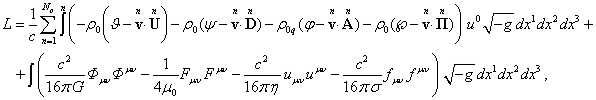
(85)

Calculating the energy , which is associated with the four-dimensional motion, as a half-sum of the relativistic energy (74) and the Lagrangian (85), we find:

(86)

where the index defines the components of 3-velocity vector of the particle with the number .

If in (57) we replace the masses and charges by the corresponding integrals in the form: , , and transform the volume units in the form , then we obtain the relation . As we can see the kinetic energy of the system in the reference frame of the center of mass vanishes, only when the velocities of all the system’s particles at the same time vanish.

We will determine the potential energy as a half-difference of the relativistic energy (74) and the Lagrangian (85):

(87)

For a solid body in the limit of the special theory of relativity, when , , , the expression for the kinetic energy (86) of the system is the following:

(88)

The main part of the kinetic energy is proportional to the square of the velocity, and vector potentials of all fields, including the velocity field and pressure field, make contribution into this part of the energy.

For the potential energy (87) of a solid body in the limit of special theory of relativity the tensor product according to (E8) tends to zero. We will also take into account the values of other tensor products:

, ,

.

It gives the following:

The potential energy depends also on the velocity. If for all material particles of the system, then the potential energy of the system remains, taking into account the field energy:

(89)

In the absence of external fields and internal motions in the fixed system in (89) the fields , , become equal to zero. As a result, with regard to (78) the potential energy becomes equal to the relativistic energy (79) for a fixed ideal solid body.

9. Conclusions

We have presented the Lagrangian of the system as consisting of one term for the curvature and four pairs of terms of identical form for each of the four fields: gravitational and electromagnetic fields, acceleration field and pressure field. As a result, for each field we have obtained equations coinciding in form with each other. The spacetime is also represented by its proper tensor metric field . The mass 4-current interacts with the specified fields, gaining energy in them, moreover the electromagnetic field changes the energy of electromagnetic 4r-current . However, the fields also have their proper energy and momentum, which are part of the tensors (5), (8), (11), (14), respectively.

The similarity of field equations implies the necessity of gauge not only of the 4- potentials of the gravitational and electromagnetic fields, but also of the 4-potentials of the acceleration field and pressure field, as well as of the mass 4-current and electromagnetic 4-current . From the standpoint of physics the meaning of such gauges is that the source of divergence of the 3-velocity vector of small volume may be the time changes in the particle’s energy in any fields which are present in the given volume. This may be the particle’s energy in the velocity field, the energy in the pressure field or the energy in the gravitational or electromagnetic fields.

In contrast to the standard approach, we do not use any of the variety of known forms of stress-energy tensors of matter. Instead, the energy and momentum of the matter are described based on the acceleration field, the acceleration field tensor and the stress-energy tensor of the acceleration field. The contribution of pressure into the system’s energy and momentum, respectively, is described through the pressure field with the help of the pressure field tensor and the stress-energy tensor of the pressure field. In this case, the acceleration field and the pressure field, as well as the electromagnetic and gravitational fields are regarded as the 4-dimensional vector fields with their own 4-potentials.

Representation of the gravitational field as a vector field is performed within the covariant theory of gravitation [3-4], in contrast to the general theory of relativity, where gravitation is described indirectly through the spacetime geometry and is considered as a metric tensor field. We consider as an advantage of our approach the fact that the energy and momentum of the gravitational field at each point are uniquely determined with the help of the stress-energy tensor of the gravitational field. Whereas in the general theory of relativity we have to restrict ourselves only to the corresponding pseudotensor, such as the Landau-Lifshitz stress-energy pseudotensor [13].

In order to uniquely identify the relativistic energy of a particle or a substance unit, we used a special gauge of the cosmological constant, giving this constant the meaning of the rest energy of the particle with “turned-off” external fields and influences. This led to the expression for the relativistic energy of the system (74) and to the equation for the metric (84), the right side of which is the sum of four stress-energy tensors of the fields.

In the absence of the cosmological constant in the Lagrangian (1) it would be impossible to perform the specified calibration, the physical system’s energy would be uncertain, and the presented theory would remain unfinished. In our approach, the cosmological constant does not reflect the energy density of the empty cosmic space, or the so-called dark energy, but rather the energy density of the matter scattered in space. Given that , where is a constant of the order of unity, it follows from (75) that . Substituting here the standard estimate of the cosmological constant m^-2, we find the corresponding mass density: kg/m. This density is sufficiently close to the density of cosmic matter, averaged over the entire space.

It can be noted that our expression for the relativistic energy and the equation for the metric differ substantially from those obtained in the general theory of relativity. For the energy it follows from the fact that instead of the stress-energy tensor of matter we use the stress-energy tensors of the acceleration field and the pressure field, while the gravitational field is directly included in the energy, and not indirectly through the metric.

Let us take the Einstein equation for the metric with the cosmological constant from [14]. In the general case, the right-hand side of this equation contains the stress-energy tensor of the electromagnetic field and the stress-energy tensor of matter :

. (90)

The simplest form of the stress-energy tensor of matter without taking into account the pressure is expression in terms of the mass density and the four-velocity: . Contraction (90) with the metric tensor gives the following:

.

where .

After substituting in (90), the equation for the metric is transformed as follows:

. (91)

Now equation for the metric (91) in the general theory of relativity can be compared with our equation for the metric (84). The main difference is that in (84) all the tensors on the right side act the same way and in contraction with the metric tensor they vanish. But it is not the case in (91) – if the expression is valid for the electromagnetic stress-energy tensor, then for the stress-energy tensor of matter the relation does not hold, so that in (91) one more term is needed. As a result, in the general theory of relativity not only the gravitational field is represented in a special way, through the metric tensor, which differs from the method of introducing the electromagnetic field into the equation for the metric, but also the stress-energy tensor of matter is not symmetric with respect to the metric, in contrast to the stress-energy tensor of the electromagnetic field .

10. References

1. C. W. Misner, K. S. Thorne, and J. A. Wheeler, Gravitation (W. H. Freeman, San Francisco, CA, 1973).

2. N. J. Poplawski, A Lagrangian description of interacting energy. – arXiv:gr-qc/0608031v2.

3. S.G. Fedosin, The Principle of Least Action in Covariant Theory of Gravitation. Hadronic Journal, 2012, Vol. 35, No. 1, P. 35 – 70.

4. S.G. Fedosin, The Hamiltonian in Covariant Theory of Gravitation. Advances in Natural Science, 2012, Vol. 5, No. 4, P. 55 – 75.

5. D. Hilbert, Die Grundlagen der Physik. (Erste Mitteilung), Göttinger Nachrichten, math.-phys. Kl., 1915, pp. 395-407.

6. H. Weyl, Raum. Zeit. Materie. Vorlesungen über allgemeine Relativitätstheorie (J. Springer, Berlin, 1919).

7. V. A. Fock, The Theory of Space, Time and Gravitation (Pergamon Press, London, 1959).

8. P. A. M. Dirac, General Theory of Relativity (John Wiley & Sons, New-York, 1975).

9. W. Pauli, Theory of Relativity (Dover Publications, New York, 1981).

10. M. Born, Die träge Masse und das Relativitätsprinzip, Annalen der Physik, Vol. 333, No. 3, 1909, pp. 571-584.

11. S. G. Fedosin, Fizicheskie teorii i beskonechnaia vlozhennost’ materii (Perm, 2009).

12. Р. Утияма, Теория относительности (М., Атомиздат, 1979).

13. L.D. Landau and E.M. Lifshitz, The Classical Theory of Fields (Vol. 2, 4th ed. Butterworth-Heinemann, 1975).

14. A. Einstein, Die Grundlage der allgemeinen Relativitätstheorie, Annalen der Physik, 1916, Vol. 354, No. 7, P. 769-822.

Appendix A. Variation of the sixth term in the action function

We need to find the variation for the sixth term in (1):

. (A1)

We will need the expressions for variation of the metric tensor and the 4-vector of the mass current, which can be found, for example, in [7], [9], [14]:

, . (A2)

. (A3)

In view of (A2) and (A3) we have the following:

(A4)

We will transform the first term in (A4) with the help of functions’ product differentiation by parts:

.

In action variation the term with the divergence can be neglected, the remaining term can be transformed as follows:

Substituting these results in (A4) and then in (A1), we find:

.

Appendix B. Variation of the seventh term in the action function

Variation for the seventh term in (1) for the special case, when is a constant, taking into account (A2) will be equal to:

,

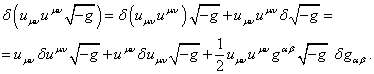(B1)

Since , the tensor is antisymmetric, then using the expression for from (A2), we find:

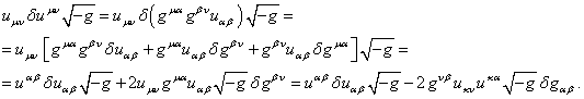
Substituting this expression in (B1) gives the following:

(B2)

We will denote by the stress-energy tensor of the acceleration field:

. (B3)

Given that , using differentiation by parts, as well as the equation which is valid for the antisymmetric tensor: , for the term in (B2) we obtain:

The term in the last expression is the divergence and it can be neglected in the variation of the action function.

Substituting the remaining term in (B2) and then in (B1) and using (B3), we find:

Appendix C. Variation of the eighth term in the action function

Action variation for the eighth term in (1) has the form:

.

Acting like in Appendix A, taking into account (A2) and (A3) we find:

.

In action variation the term with the divergence is insignificant; the second term is transformed further:

As a result, the variation of the eighth term equals:

Appendix D. Variation of the ninth term in the action function

In the special case when is a constant, for the variation of the ninth term in (1), with regard to (A2), we have:

,

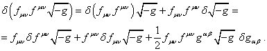(D1)

Replacing and using in (A2), we transform the first term of the equation and then substitute it in (D1):

.

We will denote by the stress-energy tensor of the pressure field:

. (D2)

We will transform the term , given that , using differentiation by parts as well as equation which is valid for the antisymmetric tensor:

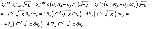
In the latter equation the term with the divergence can be neglected, since it does not contribute to the variation of the action function. Substituting the results in (D1), we find the required variation:

.

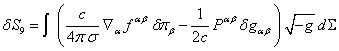Appendix E. Acceleration tensor and equations for the acceleration field

By definition, the acceleration field appears as a result of applying the 4-rotor to the 4-potential:

.

The tensor is antisymmetric and includes various components of accelerations. By its structure this tensor is similar to the gravitational tensor and the electromagnetic tensor , each of which consists of two vector components depending on the field potentials and the velocities of the field sources.

In order to better understand the physical meaning of the acceleration field, we will introduce the following notations:

, , (E1)

where the indices form triples of nonrecurring numbers of the form 1,2,3 or 3,1,2 or 2,3,1; 3-vectors and can be written by components: ; .

Then the tensor can be represented as follows:

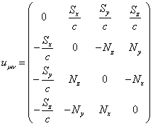. (E2)

In order to simplify our further arguments, we will consider the case of the flat spacetime, i.e. Minkowski space or the spacetime of the special theory of relativity. The role of the metric tensor in this case is played by the tensor , the non-zero components of which are , . With its help we will raise the indices of the acceleration tensor:

. (E3)

We will expand the 4-vector of the mass current: , where . In equations (22) and (23) we can replace the covariant derivatives with the partial derivatives . Now with the help of the vectors and these equations can be presented as follows:

, , , . (E4)

The equations (E4) obtained in the framework of the special theory of relativity for the case are similar by their form to Maxwell equations in electrodynamics.

If we multiply scalarly the second equation in (E4) by and multiply scalarly the fourth equation by and sum up the results, we will obtain the following:

. (E5)

Equation (E5) contains the Poynting’s theorem applied to the acceleration field. The meaning of this differential equation is that if in a system the work is done to accelerate the particles, then the power of this work is associated with the divergence of the acceleration field’s flux and the change in time of the energy associated with the acceleration field. The relation (E5) in a generally covariant form according to (33) can be written as follows:

.

We will now substitute (E2) in (30) and write the scalar and vector relations for the components of the 4-acceleration :

,

. (E6)

The components of the 4 -acceleration are obtained from these relations after canceling . As we can see both vectors and make contribution to the space component of the 4-acceleration, and the vector has the dimension of an ordinary 3-acceleration, and the dimension of the vector is the same as that of the frequency.

If we take into account that the 4-potential of the acceleration field in the case of one particle can be regarded as the covariant 4-velocity, then from (E1) in Minkowski space it follows:

, . (E7)

The vector is the acceleration field strength and the vector is a quantity similar in its meaning to the magnetic field induction in electrodynamics or to the torsion field in the covariant theory of gravitation (the gravitomagnetic field in the general theory of relativity). At the constant velocity the vectors and vanish. If there are nonzero time derivatives or spatial gradients of the velocity, then the acceleration field with the components and and the acceleration tensor appear. In this case it is possible to state that the nonzero tensor in the inertial reference frame leads to the corresponding inertia forces as the consequence of any acceleration of bodies relative to the chosen reference frame.

If we substitute the tensors from (E2) and (E3) into (B3), then thus the stress-energy tensor of the acceleration field will be expressed through the vectors and . In particular, for the tensor invariant and the time components of the tensor we have:

, , . (E8)

The component after its integration over the volume in the Lorentz reference frame determines the energy of the acceleration field in the given volume, and the vector is the density of the energy flux of the acceleration field. Therefore, to calculate the energy flux of the acceleration field the vector also should be integrated over the volume.

Appendix F. The pressure tensor and equations for the pressure field

The pressure tensor is built by antisymmetric differentiation of the 4-potential :

.

We will introduce the following notations:

, , (F1)

where the indices form triples of nonrecurring numbers of the form 1,2,3 or 3,1,2 or 2,3,1; the 3-vectors and in the Cartesian coordinates have the components: ; .

In the specified notations the tensor can be represented by the components:

. (F2)

In Minkowski space the metric tensor does not depend on the coordinates and time and consists of zeros and ones. In such space the components of the tensor repeat the components of the tensor and differ only in the signs of the time components:

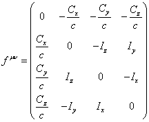. (F3)

Substituting in equations (26) and (27) the covariant derivatives with the partial derivatives , we can represent these equations in the form of four equations for the vectors and :

, , , . (F4)

We will remind that the equations (F4), obtained in the framework of the special theory of relativity, are valid for the case of . Similarly to (E5), we obtain the equation of local pressure energy conservation:

.

This equation also follows from equation (34) and can be written with the help of the tensor according to (D2) as follows:

.

Tensor invariant and the time components of the tensor are expressed with the help of (F2) and (F3) through the vectors and :

, , . (F5)

The component of the stress-energy tensor of pressure determines the pressure energy density inside the bodies, and the vector defines the density of the pressure energy flux.

We will now estimate the quantity with the index . According to (31), this quantity determines the contribution of the pressure field into the total density of the force acting on the particle. In view of (F2) it turns out that the density of the pressure force has two components:

.

For comparison , the time component is the density of the pressure force capacity divided by the speed of light:

.

The vector has the dimension of acceleration and the vector has the dimension of frequency. These vectors with the help of (F1) and the definition of the 4-potential of the pressure field in Minkowski space can be written as follows:

, (F6)

,

where denotes the 4-velocity, is the pressure in the frame of reference associated with the particle, is the Lorentz factor and is the particle velocity.

The vector according to its properties is similar to the magnetic induction vector and the vector is similar to the electric field strength. Motionless particles do not create the vector and for the vanishing of the vector it is also necessary that the relation would not depend on the coordinates. In this case, the contribution of the pressure field into the acceleration of the particles will be zero.

Source: http://sergf.ru/ccen.htm

Scientific site