На русском языке

Bulletin of Pure and Applied Sciences, Vol. 37 D (Physics), No. 2, pp. 64-87 (2018). http://dx.doi.org/10.5958/2320-3218.2018.00013.1

The covariant additive integrals of motion in the theory of relativistic vector fields

Sergey G. Fedosin

22 Sviazeva str., apt. 79, Perm, Perm Krai, 614088, Russia

E-mail: fedosin@hotmail.com

The covariant expressions are derived for the energy, momentum, and angular momentum of an arbitrary physical system of particles and vector fields acting on them. These expressions are based on the Lagrange function of the system, are the additive integrals of motion, and are conserved over time in closed systems. The angular momentum pseudotensor and the radius-vector of the system’s center of momentum are determined in a covariant form. By integrating the motion equation over the volume the integral vector is calculated and the impossibility of treatment of the integral vector as the system’s four-momentum is proved as opposed to how it is done in the general theory of relativity. In contrast to the system’s four-momentum, which collectively characterizes the motion of the system’s particles in the surrounding fields, the physical meaning of the integral vector consists in the taking account of all the energies and energy fluxes of the fields generated by the particles. The difference between the four-momentum and the integral vector is associated not only with the duality of particles and fields, but also with different transformation laws for four-vectors and four-tensors of second order. As a result, the integral vector turns out to be a pseudovector of a special kind.

Keywords: integrals of motion; vector fields; covariant theory of gravitation; angular momentum pseudotensor; integral vector; relativistic uniform system.

PACS: 04.20.Fy; 04.40.-b; 11.10.Ef .

1. Introduction

When considering physical phenomena in the curved spacetime, such additive physical quantities as energy, momentum and angular momentum of a system of particles and fields in some cases can be conserved over time and thus can uniquely characterize the system. This explains the importance of these quantities, which are integrals of motion, in mechanics as well as in other fields of physics. In the general case, in order to calculate these quantities the Lagrange function is used, which depends on the spacetime metric and on the fields, associated with the system’s particles [1].

The text below will be devoted mainly to the vector fields used to describe phenomena in macroscopic systems with a sufficiently large number of particles. The effects of gravitation will be considered within the framework of the covariant theory of gravitation [2]. In addition to the electromagnetic field, which is a vector field by its nature, we will also consider such vector fields as the acceleration field and the pressure field [3]. The acceleration field is intended to describe in a covariant way the motion of particles; similarly, the vector pressure field determines the elastic properties of matter. If necessary, we could also take into account the dissipation field [4] and the fields of strong and weak interactions [5], as the corresponding macroscopic vector fields.

The choice of the vector fields is related to the fact that they always contain the four-potential, the field tensor and the stress-energy tensor of the field. In particular, this allows us to uniquely determine the energy of any part of the system, which is difficult, for example, in the general theory of relativity [6, 7], which is a tensor theory in regard to the gravitational field.

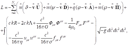
Throughout the text we will use the metric signature of the form (+, -, -, -). The initial point of our reasoning is the Lagrange function for the system of particles and four basic vector fields [8, 9]:

(1)

where is the four-potential of the gravitational field, described with the help of the scalar potential and the vector potential of this field,

is the mass four-current,

is the mass density in the reference frame associated with the particle,

is the four-velocity of a point particle, is the four-displacement, and is the interval,

 is the speed of light, as a measure of the speed of propagation of electromagnetic and gravitational interactions,

 is the four-potential of the electromagnetic field, specified by the scalar potential and the vector potential of this field,

is the charge four-current,

 is the charge density in the reference frame associated with the particle,

is the four-potential of the acceleration field, where and denote the scalar and vector potentials, respectively,

is the four-potential of the pressure field, consisting of the scalar potential and the vector potential , is the pressure in the reference frame associated with the particle, the ratio determines the equation of the state of matter,

, where is a certain coefficient of the order of unity to be determined,

is the gravitational constant,

is the scalar curvature,

is the cosmological constant,  

is the gravitational tensor (the tensor of the gravitational field strengths),

  is the definition of the gravitational tensor with contravariant indices with the use of the metric tensor ,

is the magnetic constant (vacuum permeability),

is the electromagnetic tensor (the tensor of the electromagnetic field strengths),

 is the coefficient of the acceleration field,

is the acceleration tensor, calculated as the four-curl of the four-potential of the acceleration field,

 is the coefficient of the pressure field,

is the pressure field tensor,

is the invariant coordinate three-volume, expressed in terms of the product of the differentials of spatial coordinates, and in terms of the square root of the determinant of the metric tensor taken with the negative sign.

The Lagrange function (1) can be represented in the form , that is, as the function of the radius-vectors and velocities of each of the set of particles that make up the system under consideration. With this in mind, the relativistic energy of the system, containing particles, can be determined from the formula [1]:

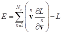, (2)

while the summation is carried out not only over all the particles, but also over all the three components of each particle’s velocity, as is required in operations with vector functions, including vector differentiation and scalar product of vectors.

The index in (2) specifies the number of a particular particle. We have placed this index over the vectors, describing the particles, in order not to confuse it with the usual indices of vectors, expressing the components of these vectors.

After substituting (1) into (2) and the energy gauging, the expression for the energy was presented in [9], both for the system of individual particles and for the case of continuously distributed matter:

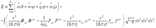(3)

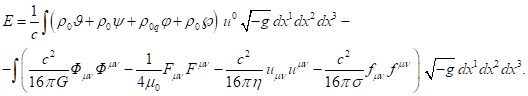(4)

In (3) the scalar potentials , , and are the quantities averaged over the particles’ volume, which are multiplied by the masses of these particles, and the results are then summed over all the particles. Since the fields can act far away from their sources, the scalar potentials include not only the intrinsic averaged potentials of the particle under consideration, but also the averaged potentials of the fields from the entire set of other particles at the location of the given particle. The quantity in (4) is the time component of the four-velocity of a typical matter particle at the point where the volume integration is carried out.

Our goal is the covariant expression of the relativistic momentum and angular momentum of the considered system of particles and four vector fields. Based on the Lagrange function and the conservation laws, we will represent the corresponding expressions in the following sections. Then we will describe the angular momentum pseudotensor, containing the system’s angular momentum and the vector defining the equation of motion of the system’s center of momentum.

In addition, we will consider the definitions of the integral vector in the general theory of relativity and in the covariant theory of gravitation. This will allow us to understand the essence of the integral vector and its fundamental distinction from the four-momentum of the system.

2. The momentum of the system

The standard approach requires that, due to the uniformity of space, the properties of the physical system must not change under any parallel transfer of this system as a whole. We will briefly recall the derivation of the law of conservation of momentum, according to [1]. Suppose that the radius-vectors of all the particles simultaneously change from to , where is a certain constant infinitesimal vector. This leads to the variation of the Lagrange function of the following form:

.

The integral of motion is obtained from the arbitrariness of choice of and from the condition of equality of the Lagrange function’s variation to zero, and hence from the condition of equality to zero of the variation action as the integral of the Lagrange function with respect to the coordinate time. This leads to the expression . Then the Lagrange equations are applied, which in our notation are written as follows:

. (5)

Substitution of the derivatives with respect to the radius-vectors by the derivatives with respect to the velocities with the help of (5) gives the following:

.

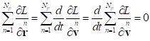
As a result, in the closed system the sum of the derivatives of the Lagrange function with respect to the velocities is conserved, which is considered as the momentum of the system:

. (6)

Let us now take into account that the Lagrange function (1), according to [9], can be represented as the sum over all the system’s typical particles as follows:

(7)

Using (7) in (6) we will find:

. (8)

The momentum (8), according to the definition in (6), is the system’s generalized momentum and is expressed in terms of the vector potentials of the fields acting on the system’s particles with masses and charges , averaged over the volume of particles. Since outside the particles there is neither mass nor charge, the vector potentials of the gravitational and electromagnetic fields outside the particles do not contribute to the system’s momentum. The quantity represents in the sum (8) the momentum of one particle with the sequential number . In the flat Minkowski spacetime, the vector potential of the acceleration field of an individual point particle equals , where denotes the Lorentz factor, is the particle’s velocity [3]. Hence we can see that the quantity in (8) really is the relativistic momentum, the contribution into which is made by the vector potentials of all the fields of the system.

For the case of continuously distributed matter, the masses and charges of the particles should be expressed, respectively, in terms of the mass density and the charge density. Let us first take into account the expression for the time component of the particle’s four-velocity: . Then, to calculate the particle’s mass it is sufficient to take the integral over its volume in the reference frame associated with the particle:

.

If the particle is moving, the element of its volume changes due to motion. Therefore, when integrating over the moving volume, an additional factor appears inside the integral. For the mass and charge of the particle it gives the following:

.

. (9)

Substituting (9) into (8) and passing from summation to integration, for the system’s relativistic momentum we find the following:

. (10)

If the fields acting in the system cannot keep the particles in equilibrium with each other, the particles’ velocities can differ to such an extent that the shape of the system will begin to change. Despite this, the energy and momentum of the closed system are conserved. These quantities are part of the system’s four-momentum:

. (11)

On the other hand, the four-momentum is defined as the product of the system’s invariant inertial mass by the four-velocity of the point, called the center of momentum of the system:

, (12)

where and specify the radius-vector and the velocity of the center of the momentum, respectively, is the coordinate time differential, denotes the proper time differential at the point of the center of momentum.

From comparison of (11) and (12) we can determine the velocity of the center of the momentum and the product of the system’s inertial mass by :

, . (13)

The value for the center of momentum should be calculated after determining the metric in the system, since , where is the interval, is the metric tensor. After that, with known energy the system’s mass can be determined from (13). Thus, the system’s energy (4) and momentum (10) with the help of (13) allow us to reduce the system’s motion to the motion of the center of momentum.

With the help of the transformation of time and coordinates, we can turn from the reference frame , in which the motion of the physical system is considered, to the reference frame , in which the system’s momentum vanishes. Such a reference frame is called the center-of-momentum frame. As a rule, in the system’s energy has the minimum value, and the four-momentum is written as follows: . In this case, according to (13), we will obtain . In the center of momentum is fixed, and therefore the possible difference between the coordinate time and the proper time at the center of momentum is caused only by the action of the fields. Thus, under the action of the gravitational field the proper time of the clock is delayed with respect to the time of the clock outside the field.

In the limit of the weak field and low velocities, the metric transforms into the metric of the flat Minkowski spacetime, in which depends only on the velocity. In this case, with the help of (13) we can estimate both the Lorentz factor of the motion of the center of momentum and the system’s mass, expressed in terms of its energy and momentum:

, .

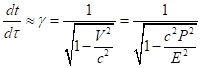3. The angular momentum of the system

For a closed system that does not interact with the environment the isotropy of space should be manifested in the fact that some property of the physical system remains unchanged during an arbitrary rotation of the system as a whole in space. Similarly to [1], we will denote the vector of the infinitesimal rotation angle of the system relative to the arbitrary axis by . The absolute value of this vector will equal , and if we look at the system from the side of the arrow of the axis and at the same time increase the angle as the system rotates counterclockwise, the vector will be directed along the axis by definition.

To find the integral of motion it is necessary to rotate the system by the arbitrary angle  and to require that the variation of the Lagrange function in this case would vanish. Rotation of the system would result in the corresponding increments of the radius-vectors and particles’ velocities, expressed in terms of the vector products:

, .

Here the second equality is obtained from the first one by differentiating with respect to the coordinate time, taking into account that behaves as a constant. Besides it is assumed that the differential and the variation do not depend on each other, so that the sequence of operations is equivalent to the sequence of operations . The particles’ radius-vectors are measured from the origin of the reference frame, which is fixed on the rotation axis, consequently the particles’ velocities are determined in the same reference frame.

For the variation of the Lagrange function after the permutation of vectors in mixed products we obtain:

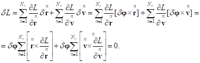
Now we’ll take into account (5):

.

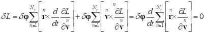Due to the arbitrariness of the vector it follows that the angular momentum vector is conserved in the closed system:

. (14)

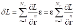
We will substitute the Lagrange function (7) into (14):

. (15)

According to (15), contribution into the total angular momentum is made by the vector potentials of all the fields, averaged over the volume of each particle of the system. At the same time the angular momentum of an individual particle is , where is the relativistic momentum of this particle, so that the angular momentum is obtained as the sum of the angular momenta of individual particles.

For the continuously distributed matter, the masses and charges of the particles in (15) should be expressed in terms of the integrals over the particles’ volume with the help of (9), and from sums we should pass to integrals. For the angular momentum it gives the following:

. (16)

The angular momentum (16) is calculated relative to the origin of coordinates of the selected reference frame. If the origin of coordinates is shifted, the radius-vectors change, so that the value of the angular momentum depends on the choice of the origin of the reference frame in contrast to the energy and momentum. Because of this the vector of the angular momentum differs from the ordinary three-vectors and is called the axial vector that behaves like a pseudovector.

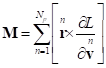
4. The angular momentum pseudotensor

In the four-dimensional spacetime, three-vectors are replaced by four-vectors and the vector product of three-vectors corresponds to the operation of antisymmetric vector product of four-vectors. The angular momentum pseudotensor for one particle with the number as a rule is defined as follows:

. (17)

For the system of particles we should sum (17) over all the particles:

. (18)

The four-dimensional radius-vector of the instantaneous position of a particle with the Cartesian spatial coordinates has the form and in the general case is not a four-vector. Instead, the differential is a four-vector. As a result, in (18) is not a tensor, but a pseudotensor, which depends on the choice of the reference frame.

Comparison of the components of the pseudotensor in (18) and the components of the angular momentum’s three-vector (15) gives the following:

, , .

This means that the components of the angular momentum of the system of particles are the space components of the angular momentum pseudotensor . As for the time components of the pseudotensor , and , they turn out to be the corresponding components of a certain three-vector . Taking into account (8) and (18) we obtain:

. (19)

In this expression the quantity represents the time component of the four-momentum of the particle with the number , is the system’s momentum. Let us introduce the radius-vector of the center of momentum of the system under consideration:

. (20)

Here the system’s energy is defined in (3) in terms of the scalar field potentials and the field tensors.

We note that the limit of weak fields and low velocities of motion of the system’s particles exists for (20). If the particles are neutral and interact weakly with each other by means of the fields, then in (3) we can neglect the second term in the form of an integral for the fields’ energy, and in the first term we can take into account only the scalar potential of the acceleration field . Then the energy of one particle will be , and for the radius-vector of the center of momentum we can write the following:

.

If we move on and neglect the Lorentz factors of the particles, then the center of momentum turns into the so-called center of mass, the radius-vector of which will be equal to:

.

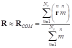Taking into account relation (20) in (19) and substituting the momentum with the help of (13) we find:

. (21)

The vector is often called a time-varying dynamic mass moment.

In a closed system the pseudotensor in (18) must be conserved, and its components must be some constants. For the space components of the pseudotensor this results in conservation of the angular momentum: . From the equality of the pseudotensor’s time components and the components of the vector in (21) it follows that it should be . It can be written as , where the constant vector specifies the position of the system’s center of momentum at . Thus, in this reference frame we obtain the equation of motion of the center of momentum at the constant velocity . In this case, the physical system has the conserved energy , momentum , angular momentum and the angular momentum pseudotensor . The constancy of the velocity follows from the constancy of energy and momentum, according to (13).

We will turn our attention to the expression for the vector in (19) and the definition of the radius-vector of the center of momentum (20). They contain the quantity , which specifies the time component of the four-momentum of a particle with an arbitrary number . Thus, it is assumed that for each particle its four-momentum is fully known. But actually only the space component of the four-momentum is most easily determined in the form of the particle’s momentum , since the vector potentials of the fields can be found from the solution of the fields’ equations. As for particle energy , here we have a problem related to the field energy, which should be taken into account in . Indeed, from the formula for the system’s energy (3) it follows that contribution into the system’s energy is made, with the help of the integral, by the fields – both inside the system and beyond its limits, up to infinity. Apparently the fields’ energy must be somehow included in the energy of each particle of the system, but it is not easy, since the fields’ energy in (3) has an integral form and cannot be divided exactly into the contributions from individual particles.

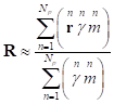
In this connection, at the first glance it seems that the definition of the radius-vector of the center of momentum (20) has a formal character. Nevertheless, with the help of it can be satisfactorily estimated in case, when the fields’ energy is small in comparison with the energy of particles in the scalar field potentials acting on them. If the particles’ velocities are known, we can use the first relation in (13) and approximately find the particles’ energies with the known momenta. Similarly, if we know the masses and the quantities for each particle, then using the second relation in (13) we can estimate the energies of individual particles, and then substitute them into (20). All this gives the following for the radius-vector of the center of momentum:

, . (22)

For the case of the continuously distributed matter, all the sums included in the definition of the angular momentum pseudotensor are replaced by the integrals, since instead of the masses and charges of particles the products of the mass density and charge density by the volume of typical particles are used. In this case, the pseudotensor’s space components will be the components of the angular momentum of the system of particles, according to (16). The pseudotensor’s time components are represented by the components of the vector and, according to (21), they remain unchanged. This follows from the definitions:

, , (23)

where denotes the differential of the integral taken over the volume, is the four-momentum of the system (11).

To complete the picture, we will express the time and space components of in (23) with the help of expressions for the energy (4) and momentum (10) of the system:

.

Here the index specifies the space components of the system’s four-momentum, which are, respectively, the three components of the three-momentum vector . In particular, for the Cartesian coordinate system , , .

To determine the radius-vector of the center of momentum in case of the continuous distribution of matter, in the first approximation, the second relation in (22) can be used. Taking into account that , where is the time component of the four-velocity of the particle with the number , and passing from summation to integration, we find:

. (24)

Here the system’s energy is given by relation (4). In the course of derivation of (22) we pointed out that the contribution to the energy of individual particles should also be made by the fields present in the system. This also applies to (24). The problem here is that the interacting particles themselves are not closed systems, but they are immersed in the common force fields acting on these particles at a distance and changing their energies and momenta. For an unclosed system in the external field in the form of a single particle inside the considered system of particles and fields, application of (4) for integration over the volume of this particle gives the energy of a part of the entire system of particles and fields in this volume, but not the energy of the particle as such.

In this connection, we should refer to the initial formula (20) to estimate the radius-vector of the center of momentum. In order to simplify the situation, we will assume that the closed system under consideration has an axisymmetric configuration with respect to the energy distribution of the particles and fields. Then we can see that the resultant contributions of the fields, going beyond the system’s limits, into the value and direction of the vector become zero due to the symmetry of the system configuration. No matter how the energies of the external fields change the particles’ energies in (20) as compared to the energies of free particles with the same particles’ motions, the value remains the same. Therefore, in (20) it will suffice to take into account the particles’ energies in the scalar field potentials and the fields’ energies in the volume of typical particles. Passing from summation to integration over volume and using (4) we find the following:

(25)

According to the above reasoning, for the axisymmetric configurations in (25) it is not necessary to integrate over the space outside the system, where there is no matter.

On the other hand, we can imagine such physical systems, in which the main role is played by the energy of fields, rather than the energy of the matter particles. For example, the system can consist of a number of charged capacitors, in each of which there is a strong electric field. Each energy has inertia and the corresponding mass, so that the motion of the system with capacitors gives rise to the system’s momentum, and rotation of the system also causes the angular momentum. In this case, the second integral with the fields’ energies in (25) becomes of primary importance. Consequently, unit space volumes, containing fields both inside and outside the system up to infinity, can be considered as particles of a special kind, making their contribution to determination of the radius-vector of the system’s center of momentum . This means that (25) should hold true not only for axisymmetric systems, but also for systems of any form. Therefore, in the general case, integration in the second integral in (25) should be carried out over the entire infinite volume.

These arguments can be extended to the expressions for the energy in (4), for the momentum in (10) and for the angular momentum in (16), in case of continuous distribution of matter. In this case, these expressions actually become additive integrals of motion, since each small part of space in them contains either matter and fields or only fields, and makes its contribution into the system’s integrals of the motion.

5. The situation in the general theory of relativity

Being a tensor theory, the general theory of relativity (GTR) differs significantly from the vector covariant theory of gravitation (CTG). Firstly, the gravitational field in GTR has neither its own four-potential nor the field tensor, instead of it all gravitational effects are expressed in terms of the metric tensor and its derivatives. Secondly, the acceleration field in GTR is presented not as a vector field, but as a simpler scalar field, and it does not have its own tensor either. This can be seen from the Lagrange function used in GTR [10]. In our notation this function is written as follows:

. (26)

Here , where ϰ is the Einstein’s gravitational constant.

In (26) the last term specifies the contribution into the Lagrange function from the elastic energy of matter, and if this energy is associated with the pressure field, then, as a rule, this field is considered in GTR not as a vector field, but as a simple scalar field.

By definition, the four-velocity is gauged in such a way that , so that hence the definition follows for the square of the interval in the form . In this connection, the scalar invariant quantity in (26) can also be written as [11, 12], while in [8] and [13] the product is used for this, where is the mass four-current. In contrast to this, instead of the quantity , in the framework of CTG we use in (1) the acceleration field invariant in the form of ; in this case the vector nature of the acceleration field is emphasized by the additional invariant , which contains the acceleration tensor .

Let us now consider how the relativistic energy, momentum and angular momentum of the system of particles and associated fields are calculated in GTR. Thorough analysis shows that in GTR there are no formulas that determine the given quantities in the curved spacetime in an exact and covariant way. We have already referred to the articles [6, 7], which prove the impossibility of unambiguous calculation in GTR of the energy and mass of any arbitrarily chosen small part of the system. First of all this is due to the fact that in GTR the gravitational field is represented in the Lagrange function not directly, but indirectly, through the scalar curvature , expressed in terms of the metric tensor and its derivatives. To estimate the contribution of the energy and the energy flux of the gravitational field in the generalized Poynting theorem, the corresponding stress-energy tensor should be used for the system under consideration. However, instead of it, we can only find the stress-energy pseudotensor of the gravitational field, usually for the case when the cosmological constant is zero. In this case, the form of this pseudotensor cannot be unambiguously defined. For example, the Einstein pseudotensor is well-known, which, according to [14], in sum with the stress-energy tensor of matter and non-gravitational fields should give the conservation law of the following form:

. (27)

It is assumed that integration over the infinite three-dimensional volume of the tensors’ time components in (27) leads to the four-momentum of the system with regard to the contribution of the energy and momentum of the gravitational field:

. (28)

The index in shows that the integral vector is calculated with the help of the Einstein pseudotensor.

As is indicated in [13], in the general case it is impossible to fulfill simultaneously two conditions for a closed system with the help of the quantity :

1) conservation over time of the sum of all the types of energy, including the gravitational energy defined by the pseudotensor ;

2) independence of the sum of all the types of energy at a given time point from the choice of the reference frame.

In addition, unlike the tensor , the pseudotensor is asymmetric and therefore the integral vector cannot be used to calculate the relativistic angular momentum of the system. To solve this problem Landau and Lifshitz invented [15] the symmetric gravitational field pseudotensor , so that the following relation holds true:

. (29)

The integral over the infinite volume gives the following:

. (30)

It is assumed that the integral vector is also the system’s four-momentum. To substantiate this conclusion, we need to send the pseudotensor to zero in (30), then would tend to the system’s four-momentum without taking into account the contribution of the gravitational field. In this case, it seems that should give the four-momentum with regard to the contribution of the gravitational field.

Landau and Lifshits also find the system’s angular momentum with the help of the integral over the infinite volume. To do this, they determine the four-dimensional pseudotensor of the angular momentum as the integral over the volume taken of the vector product of the current four-dimensional radius-vector by the integral vector differential associated with a given point in space:

.

(31)

The need to integrate over the infinite volume in (28), (30) and (31) is related to the fact that the gravitational field pseudotensor does not specify the unique distribution of gravitational energy and momentum in the considered physical system, which does not depend on the choice of the reference frame. It is assumed that integration over the entire volume allows us to minimize the possible inaccuracies arising from this circumstance. At the same time, by choosing the appropriate reference frame we can achieve that at infinity the metric of the physical system would turn to the metric of the flat spacetime. In this case, the pseudotensor vanishes at infinity, as it should be for the gravitational interaction.

In case if the cosmological constant is taken into account in (26), in (29) the gravitational field pseudotensor should be replaced by , and the corresponding additions should be made in (30) and (31). Similarly, according to [16], the pseudotensor in (27) should be replaced by , and in (28) should be substituted by .

The above-mentioned pseudotensors of the gravitational field contain only the metric tensor and its first-order derivatives. In theory it is possible that there are many other gravitational field pseudotensors, which, summed up with the stress-energy tensor , could give the conservation laws similar to (27) or (29). We will not go deep into the history of this problem and describe other known pseudotensors, since our goal was to illustrate the very fact of ambiguity in the choice of pseudotensor for the conservation law in GTR. References to other pseudotensors and related problems can be found, for example, in [17].

In opinion of the authors in [18], who analyzed the conservation law (27), if the necessary conditions (integration over the infinite volume, the system “being immersed” into the Minkowski space at infinity) are met, the quantity in (28) must be identically equal to zero and therefore cannot be the four-momentum and specify the inertial mass of the system. They also pay attention to different transformation laws for the matter tensor and the gravitational field pseudotensor . This should lead to different values of in different reference frames, which contradicts the condition of independence of the physical system’s inertial mass from the choice of the reference frame. In connection with this, in [7] such quantities as in (28) and in (30) are considered not as four-vectors, but as pseudovectors. In [6] it is emphasized that GTR does not satisfy the correspondence principle in the sense that the expression for the inertial mass in the general case in the limit of the weak field and low velocities does not go over to the corresponding expression in the Newton’s theory. According to [19], the correspondence principle in GTR is not satisfied for all the additive integrals of motion, including energy, momentum, and angular momentum.

The considerations presented above raise doubts that in the general theory of relativity it is possible to uniquely determine the energy, momentum, inertial mass and momentum of the considered physical system. At least it is absolutely impossible in case if it is necessary to calculate these quantities for an individual arbitrarily chosen internal part of the system. We will return to the discussion of this question in the conclusion of this paper, after presentation of the integral vector from the perspective of the vector field theory.

6. The integral vector

The equation used to find the metric tensor components in the covariant theory of gravitation for the tensors with mixed indices has the following form [9]:

. (32)

here is the Ricci tensor with mixed indices; is the unit tensor or the Kronecker symbol; , , and are the stress-energy tensors of the gravitational and electromagnetic fields, acceleration field and pressure field, respectively.

With the help of the covariant derivative we can find the four-divergence of both sides of (32). The divergence of the left-hand side is zero due to equality to zero of the divergence of the Einstein tensor, , and also as a consequence of the fact that outside the body the scalar curvature vanishes, , and inside the body it is constant. The latter follows from the gauge condition of the energy of the closed system. The divergence of the right-hand side of (32) is also zero:

. (33)

The tensor with mixed indices represents the sum of the stress-energy tensors of all the fields acting in the system. Expression (33) for the tensors’ space components is nothing but the differential equation of the matter’s motion under the action of forces generated by the fields, which is written in a covariant form. As for the tensors’ time components, for them expression (33) is the expression of the generalized Poynting theorem for all the fields.

If we could integrate (33) over the four-dimensional volume, then as a result an additive integral of motion could be obtained. In this case it should be taken into account that the situation inside and outside the particles or inside and outside the continuously distributed matter differs significantly. Indeed, in the space where there is no matter, there are only the electromagnetic and gravitational fields. In the matter the acceleration field and the pressure field are also acting. Therefore, integration over the volume in (33) should be divided into two parts – one integration over the volume for the matter particles (or for the typical particles of continuously distributed matter), and the second one for the space outside the matter.

Since is a symmetric tensor, its covariant derivative has the following representation:

. (34)

Since gravitation is considered in the covariant theory of gravitation as an independent entity that does not require justification through the metric, the gravitational effects do not disappear even in the flat Minkowski spacetime. The same is true for the electromagnetic field and its effects. In Minkowski spacetime, the metric tensor does not depend on the coordinates and time, and , as well as . Consequently, (34) is simplified and in the weak field and at low velocities of particles we can write:

.

This expression can be integrated over the four-volume, taking into account the Gauss’ theorem:

,

where denotes an element of some three-dimensional hypersurface that surrounds the four-volume under consideration.

In a closed system, the integral vector must be constant. In order to get a general idea of the vector it is enough to determine its instantaneous value at . For example, if , we can take the initial time point . In the standard gauge, the origin of time and the origin of space coordinates at the initial time point (the center of momentum of the closed physical system, moving at velocity ) intersects the origin of the observer’s reference frame. Then for the integral vector we can write the following:

. (35)

Let us now consider the simplest macroscopic physical system in the form of a sphere, which is filled with randomly moving charged typical particles so densely that the approximation of continuous medium can be applied. These particles are held inside the sphere by the gravitational field. We will now use the solutions known for such a system in the framework of the relativistic uniform model that takes into account the vector gravitational and electromagnetic fields, as well as the acceleration field and the pressure field. Let the origin of the reference frame be at the center of the sphere, so that we will search in the reference frame where the sphere is stationary.

If we take into account the randomness of the typical particles’ motion in each sufficiently large volume element, then we can see that the global vector potentials of all the fields inside and outside the sphere on the average are equal to zero. This leads to the fact that all the global solenoidal vectors are also equal to zero, and in particular the magnetic field and the gravitational torsion field on the average are equal to zero, according to the covariant theory of gravitation. Consequently, in the given physical system, which is stationary relative to the selected reference frame, there are no energy fluxes (momentum fluxes) of the fields, calculated with the help of the vector products of the field strengths by the corresponding solenoidal vectors.

In view of (33) , while at the index values the components are proportional to the sums of the energy fluxes of individual fields. In the case under consideration, the fields’ energy fluxes, such as the Poynting vector or the similar Heaviside vector for the gravitational field, are absent, and in (35) only one nonzero time component of the integral vector is left at the index value :

. (36)

We will now take into account the explicit expressions for the stress-energy tensors of the gravitational field [2], [8], the electromagnetic field, the acceleration field and the pressure field [3], [9], derived from the principle of least action:

,

,

,

. (37)

As we can see from (36) and (37), in order to obtain it is necessary to integrate over the volume the sum of the time components of the stress-energy tensors of all the fields, that is, the sum of the energy densities of these fields. In the flat Minkowski spacetime and at zero solenoidal vectors, the fields’ energy densities depend only on the strengths of the fields, which are part of the tensors of the corresponding fields. For example, in case the magnetic field is equal to zero the electromagnetic tensor depends only on the electric field strength , and the following expression is obtained for the energy density of the electromagnetic field: .

Likewise, for the energy densities of the gravitational field, the acceleration field and the pressure field at solenoidal vectors equal to zero, we obtain [9], [20]:

, , , (38)

where , and denote the strengths of the gravitational field, the acceleration field and the pressure field, respectively. In this case, the expressions for the field strengths inside the sphere in the spherical coordinates depend only on the current radius , and the radial components of the field strengths have a similar form [21]:

,

,

,

(39)

In (39) is the Lorentz factor of the typical particles that are in motion at the center of the sphere. Substituting (39) into (38), and substituting the results into (36), we find inside the sphere by integrating over the volume in the spherical coordinates the following:

. (40)

As was found in [22], by virtue of the equation of motion of the typical particles inside the sphere, in the case under consideration the following relation holds true:

.

If we take this expression into account in (40), we can see that the time component of the integral vector inside the sphere vanishes: .

The radial components of the strengths of the gravitational and electromagnetic fields outside the sphere with radius are equal [20]:

,

,

(41)

where is the gravitational mass of the system, is the total charge of the system. In this case, the inertial mass of the system in (13) differs from the gravitational mass . This is due to the fact that the inertial mass is calculated through the relativistic energy of the system (4) by formula (13) and takes into account the contributions from all the particles and fields of the system, while the gravitational mass is equal to the total mass of the particles from which the system was formed. Likewise, the charge is the total charge of the particles from which the system was formed.

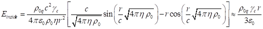
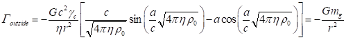
With the help of (41) we can calculate the expressions for and in (38). Substituting these tensor components into (36), for the time component of the integral vector outside the sphere we find the following:

. (42)

Adding up (40) and (42), for the time component of the integral vector we have:

. (43)

Now we can understand the essence of the integral vector in (35). This vector, which is an integral over the four-volume at the initial time point taken of the equation of motion written in the form of (33), shows the distribution of the energy and energy fluxes in the closed system. When the system as a whole is moving relative to the external observer, the vector is a function of coordinates and time, the same applies to the potentials and strengths of all the fields. If the origin of the reference frame is moving synchronously with the center of momentum, then in such a reference frame the integral vector depends only on the internal motion of the particles and fields of the physical system. The vector obtains the simplest form in case if the center of momentum always coincides with the origin of the reference frame, that is, at the center of momentum.

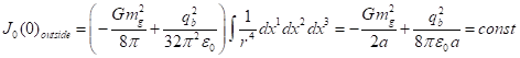
According to (43), in the physical system, which is stationary on the average, when there are no global mass and charge currents in the matter, only the time component of the integral vector is not equal to zero. In this case, within the framework of the relativistic uniform model, is equal to the sum of the energies of the gravitational and electric fields outside the matter. As for the volume inside the system’s matter, here the sum of contributions of the energies of all the fields vanishes. For the nonzero space components of the integral vector to appear in (35) at index values , some stationary motion of the matter and fields is required, for example, general rotation, volume pulsations or mixing of matter. In this case, solenoidal vectors and the fields’ energy fluxes appear in the system.

It is obvious that in the long-term perspective the integral vector will not be conserved over time even in a closed system if it does not take into account the contribution of the vector dissipation field, as it was done, for example, in [4]. In real systems, there is always dissipation of energy and transformation of the energy of motion of the particles’ fluxes into thermal energy. This leads to a change in the state of the matter fluxes in the system until the equilibrium state is achieved, when the gradients of the matter particles’ velocities in the adjacent fluxes reach the minimum. At the same time, there is a change in the fields’ energy fluxes, and, consequently, in the integral vector’s components.

7. Conclusion

The initial point of our reasoning in the definition of additive integrals of motion was the expressions for the Lagrange function (1) for the continuous distribution of matter, as well as for the Lagrange function (7) in case when the matter consists of individual particles. With the help of these expressions, using the standard procedure we find formulas (3) and (4) to determine the relativistic energy of the system for the case of individual particles and for the case of continuous distribution of matter, respectively, formulas (8) and (10) to determine the relativistic momentum , formulas (15) and (16) to determine the relativistic angular momentum . With the help of the energy and the momentum it becomes possible to determine the system’s four-momentum in (11).

Since the angular momentum depends on the choice of the reference frame, it is a three-dimensional pseudovector. Similarly, the angular momentum tensor in (18) and in (23) is actually a four-dimensional pseudotensor, since it contains both the components of the pseudovector and the components of the vector in (21). The vector defines the equation of motion of the center of momentum of a closed system at a certain constant velocity, while the radius-vector of the center of momentum is determined in a covariant form in (25).

In section (5) we briefly describe how the integrals of motion are defined in the general theory of relativity (GTR). Analysis of the situation shows that in GTR the system’s energy depends on the stress-energy pseudotensor of the gravitational field, the values of which at each point depend on the choice of the reference frame. Moreover, the existence of many different forms of the stress-energy pseudotensor of the gravitational field suggests that in GTR it is impossible to uniquely calculate the energy in any given small volume inside the system. Nevertheless, it is asserted that the integral vectors such as (28) or (30) obtained by integration over the infinite volume give the energy and momentum of the system. Unfortunately, this heuristic conclusion does not follow from the standard procedures and the physico-mathematical logic of the field theory.

Indeed, in order to show that the integral vector in the weak-field limit tends to the four-momentum of the system, it is necessary to send the gravitational field pseudotensor to zero, and to send the curved spacetime metric to the Minkowski spacetime metric. In this limiting case, according to GTR, the gravitational effects must disappear completely, and all physical systems must behave like inertial reference frames. Thus, the ideal inertial frames in GTR must be without mass and charge, otherwise they would generate gravitational and electromagnetic fields, and therefore the metric tensor would also change.

Now we can raise a question: is it actually possible to send the gravitational field pseudotensor to zero in any system at all? Apparently, it is possible only if at the same time we remove from the system the matter that carries the mass and charge. But when the pseudotensor is zeroed, neither mass nor charge would remain in the system, and the four-momentum of the system would become equal to zero. But this is the only state of the system, in which we can be absolutely sure. If the system has both the mass and the gravitational field pseudotensor, then there is no guarantees that the integral vector in GTR defines precisely the four-momentum of the system.

In addition, in GTR the pressure field is used not as a vector field, but as a scalar field, and the same applies to the acceleration field. As a result, in GTR the energy and energy fluxes of these fields are not fully taken into account in the integral vector. Meanwhile, at equilibrium, the gravitational and electromagnetic fields, the acceleration field and the pressure field in the matter inside the system, which is stationary in general, are such that they completely balance each other. This means that all the forces applied to each typical particle of matter on the average are equal to zero. Moreover, our approach, in view of the covariant theory of gravitation and the four acting fields, shows that in the matter the sum of the energies of all the fields, as well as the time component of the integral vector become equal to zero, according to (40). Only the energy of the fields (43) that go out of the system beyond the matter’s limits contributes to the integral vector of such a system. As a result, the integral vector is associated with the energies and energy fluxes in the system, but not with the four-momentum of the system. The same must be true for the integral vector in GTR, since it is also obtained by integrating over the four-volume of the divergence taken from the stress-energy tensor of the matter and non-gravitational fields with addition of the gravitational field pseudotensor. In this connection, consideration of the integral vector as the four-momentum in GTR in our opinion is wrong. Other problems, associated with considering the integral vector as the four-momentum in GTR, are described above in Section 5 with the appropriate references.

The difference between our integral vector and the four-momentum is significant and consists in the fact that in the center-of-momentum frame the system’s momentum and the space vector component are equal to zero and reflect the motion of the matter’s particles in the vector field potentials. This follows from the definition of in (8) and in (10), where either mass and charge or the densities of mass and charge of the particles are present. As for the space vector component of the integral vector , it is associated with the motion of the fields rather than particles, that is, with the fields’ energy fluxes contained in the stress-energy tensors of the fields. The same can be said about the time components – if in the time component is associated with the relativistic energy of the particles in the scalar potentials with the addition from the fields’ energy, then in the time component is calculated using the energy densities contained in the stress-energy tensors of the fields. As we can see, the methods of calculation of and differ significantly from each other: in order to find we need the four-potentials of the fields, and in order to find in (35) we necessarily need the stress-energy tensors of all the fields. It turns out that the difference between and is due to the fundamental difference between particles and fields, they cannot be reduced to each other, although they are interrelated with each other.

Another peculiarity is that in an arbitrary reference frame the system’s momentum , as well as the space vector component are no longer equal to zero and reflect the property of inertia as resistance to the force changing the momentum . And what is the meaning of the space vector component of the integral vector in an arbitrary reference frame? Since is the integral vector taken at the initial time point, it reflects only the configuration of the energy and the fields’ energy fluxes of the system at this time point and the corresponding fields’ momentum. For example, we can take a rotating body that, when moving as a whole, has not only the four-momentum , but also has the integral vector with nonzero space components due to the fields’ energy fluxes arising from rotation and linear motion. In this case, in the closed system at equilibrium the fields’ energy fluxes in the matter and beyond its limits become closed.

Finally, it should be mentioned that the integral vector in principle cannot be the system’s four-vector and four-momentum. This follows from the fact that according to (12) the four-momentum can be defined as the product of the system’s inertial mass by the system’s four-velocity: . This definition is valid in any reference frame. However, such a definition for the integral vector is unsuitable. The basis of the proof here is the so-called 4/3 problem. The essence of the electromagnetic field is that the field’s mass-energy of the moving charged body, calculated at the initial time point by integrating the component of the stress-energy tensor of the electromagnetic field over the volume, is approximately 4/3 times less than the field’s mass-energy, calculated in the initial time point by integrating the space components of the stress-energy tensor over the volume.

The existence of the 4/3 problem, that is, non-coincidence of the above-mentioned mass-energies, stems from the fact that the four time components of the stress-energy tensor of the electromagnetic field do not constitute any four-vector in total, and they are transformed from one reference frame to another by the tensor law rather than by the vector law. The same is true for the gravitational field in the covariant theory of gravitation [23], and for any vector fields with the four-potential in general. Since the integral vector is the integral over the volume of the sum of the time components of the fields’ stress-energy tensors, the integral vector is not a four-vector either. This can be proved directly, for which it is sufficient to recalculate the time component  in (43), but already for a moving system at the initial time point. This component of the integral vector will increase due to the system’s motion at velocity  by a factor of about , where is the Lorentz factor. At the same time, the system’s energy, which is part of the time component of the four-momentum , under the same conditions will increase only by a factor of .

Consequently, the integral vector in (35) is a four-dimensional pseudovector, but not the system’s four-momentum. Indeed, the integral over the volume of the differentials of four-momentum can give the four-momentum of the system, but this cannot be expected from the integral over the volume of the time components of the system’s stress-energy four-tensor, due to different transformation laws for four-vectors and four-tensors of second order.

The fact that the integral vector is a four-dimensional pseudovector makes it close in the meaning to another additive integral of motion of the system and to a three-dimensional pseudovector, namely the angular momentum . If desired, like Landau and Lifshitz with the help of we could introduce the momentum pseudotensor of the integral vector, similarly to (31). However, according to the foregoing, this pseudotensor would not be equal to the system’s angular momentum pseudotensor in (18) and (23), but would characterize only the angular momentum of the fields’ energy fluxes.

References

1. Landau L.D., Lifshitz E.M. (1976). Mechanics. Vol. 1 (3rd ed.). Butterworth-Heinemann. ISBN 978-0-7506-2896-9.

2. Sergey Fedosin, The physical theories and infinite hierarchical nesting of matter, Volume 2, LAP LAMBERT Academic Publishing, pages: 420, ISBN-13: 978-3-659-71511-2. (2015).

3. Fedosin S.G. The procedure of finding the stress-energy tensor and vector field equations of any form. Advanced Studies in Theoretical Physics, Vol. 8, pp. 771-779 (2014). doi:10.12988/astp.2014.47101.

4. Fedosin S.G. Four-Dimensional Equation of Motion for Viscous Compressible and Charged Fluid with Regard to the Acceleration Field, Pressure Field and Dissipation Field. International Journal of Thermodynamics, Vol. 18, No. 1, pp. 13-24 (2015). doi: 10.5541/ijot.5000034003.

5. Fedosin S.G. The Concept of the General Force Vector Field. OALib Journal, Vol. 3, pp. 1-15 (2016), e2459. doi:10.4236/oalib.1102459.

6. Denisov V.I., Logunov A.A. The inertial mass defined in the general theory of relativity has no physical meaning. Theoretical and Mathematical Physics, Vol. 51, Issue 2, pp. 421-426 (1982). doi:10.1007/BF01036205.

7. Khrapko R. I. The Truth about the Energy-Momentum Tensor and Pseudotensor. Gravitation and Cosmology, Vol. 20, No. 4, pp. 264-273 (2014). doi:10.1134/S0202289314040082.

8. Fedosin S.G. The Principle of Least Action in Covariant Theory of Gravitation. Hadronic Journal, Vol. 35, No. 1, pp. 35-70 (2012). doi:10.5281/zenodo.889804.

9. Fedosin S.G. About the cosmological constant, acceleration field, pressure field and energy. Jordan Journal of Physics, Vol. 9, No. 1, pp. 1-30 (2016}. doi:10.5281/zenodo.889304.

10. Fock V.A. The Theory of Space, Time and Gravitation. (Pergamon Press, London, 1959).

11. Hilbert D. Die Grundlagen der Physik. (Erste Mitteilung), Göttinger Nachrichten, math.-phys. Kl., 1915, pp. 395-407.

12. Weyl H. Raum. Zeit. Materie. Berlin, J. Springer. 1919.

13. Dirac P.A.M. General Theory of Relativity (1975), Princeton University Press, quick presentation of the bare essentials of GTR. ISBN 0-691-01146-X.

14. Einstein A. Das hamiltonisches Prinzip und allgemeine Relativitätstheorie (The Hamiltonian principle and general relativity). Sitzungsber. preuss. Acad. Wiss. Vol. 2, 1111-1116 (1916).

15. Landau L.D., Lifshitz E.M. The Classical Theory of Fields, (1951). Pergamon Press. ISBN 7-5062-4256-7, chapter 11, section #96.

16. Pauli W. Theory of Relativity (Dover Publications, New York, 1981).

17. M. Sharif, Tasnim Fatima. Energy-Momentum Distribution: A Crucial Problem in General Relativity. Int. J. Mod. Phys. A, Vol. 20, p. 4309 (2005). doi:10.1142/S0217751X05020793.

18. Denisov V.I., Logunov A.A. Further remarks on the inequlity of the inertial and gravitational masses in general relativity. Theoretical and Mathematical Physics, Vol. 85, Issue 1, pp. 1022-1028 (1990). doi:10.1007/BF01017242.

19. Denisov V.I., Logunov A.A. Does the general theory of relativity have a classical Newtonian limit? Theoretical and Mathematical Physics, Vol. 45, Issue 3, pp. 1035-1041 (1980). doi:10.1007%2FBF01016702.

20. Fedosin S.G. The Integral Energy-Momentum 4-Vector and Analysis of 4/3 Problem Based on the Pressure Field and Acceleration Field. American Journal of Modern Physics. Vol. 3, No. 4, pp. 152-167 (2014). doi:10.11648/j.ajmp.20140304.12.

21. Fedosin S.G. Relativistic Energy and Mass in the Weak Field Limit. Jordan Journal of Physics. Vol. 8, No. 1, pp. 1-16 (2015). doi:10.5281/zenodo.889210.

22. Fedosin S.G. Estimation of the physical parameters of planets and stars in the gravitational equilibrium model. Canadian Journal of Physics, Vol. 94, No. 4, pp. 370-379 (2016). doi:10.1139/cjp-2015-0593.

23. Fedosin S.G. 4/3 Problem for the Gravitational Field. Advances in Physics Theories and Applications, Vol. 23, pp. 19-25 (2013). doi:10.5281/zenodo.889383.

Source: http://sergf.ru/caen.htm

Scientific site