Canadian Journal of
Physics, Vol. 93, no. 11, P. 1335-1342 (2015). http://dx.doi.org/10.1139/cjp-2015-0134
The Pioneer Anomaly in Covariant
Theory of Gravitation
Sergey G. Fedosin
Sviazeva Str. 22-79, Perm, 614088, Russian
Federation
e-mail intelli@list.ru
Abstract: The difference of
equations of motion in
the covariant theory of gravitation and in the general theory of relativity is
used to explain the Pioneer anomaly. Calculation
shows that the velocities of a spacecraft in both theories at equal distances
can differ by several centimetres per second. This
leads also to a possible explanation of the flyby anomaly and comet disturbances
which are not taken into account by the general theory of relativity.
Keywords: Pioneer anomaly, covariant theory of gravitation, general theory of relativity, equation of motion, flyby anomaly.
PACS: 04.50.Kd, 04.20.Jb, 04.80.-y,
95.55.Pe
Résumé: Les differences entre les équations de mouvement dans la théorie covariante de la
gravitation et dans la théorie générale de la
gravitation sont utilisées
pour expliquer “l'anomalie
Pioneer”. Le calcul montre que les vélocités des sondes spatiales dans les deux theories aux
distances différentes peuvent
se différencier à plusieurs
cm/s. Cela amène à l’explication possible de l'anomalie
“flyby” et aux perturbations de la comète
qui ne sont pas pris en compte dans la théorie générale de la relativité.
1. Introduction
The stories of the
American spacecrafts Pioneer 10 and Pioneer 11 began on 2 March 1972, and, respectively, on 6 April
1973, respectively, at the times of their launches. Both spacecrafts passed in
the ecliptic plane of the entire Solar system in opposite directions, passing
close to different planets. Pioneer 10 on 4 December 1973, reached Jupiter,
located at a distance of 5.2 a.u. from the Sun (1 a.u. = 1.496·1011 m), in June 1983 it passed
Pluto (39.4 a.u.), in May 2001 it was at the distance
of 78 a.u., moving at a speed of nearly 13 km/s.
Starting from a distance
of about 20 a.u., when it was evident from the
Doppler signal from Pioneer 10 that the shift of the speed significantly decreased,
caused by the pressure of the solar plasma on the spacecraft, after taking into
account all other possible causes of acceleration, the residual signal from the
spacecraft started to show the presence of an anomalous acceleration towards
the Sun, of the order of 8·10–10 m/s2 [1]. For Pioneer 11
a similar acceleration was of about 8.6·10–10 m/s2; for
the spacecraft Ulysses at distances of 1.3 – 5.2 a.u.
the acceleration reached (12 ± 3)·10–10 m/s2,
while for the spacecraft Galileo – 8·10–10 m/s2.
There are some possible explanations
for anomalous acceleration of the spacecrafts. One of them for the Pioneer 10
and 11 spacecraft is due to the recoil force associated with an anisotropic
emission of thermal radiation off the vehicles [2-3]. The other explanations of
the Pioneer anomaly include new gravitational physical mechanisms [4-10].
The covariant theory of
gravitation (CTG) is an alternative theory to the general theory of relativity
(GTR) and we present further CTG approach to the problem of the Pioneer anomaly
by comparing of calculations of CTG and GTR.
2. Metric tensor in CTG
The metric tensor in
spherical coordinates ![]() ,
, ![]() ,
, ![]() ,
, ![]() has the following form:
has the following form:
 , (1)
, (1)
and for the functions ![]() we assume that they are the functions only of
the radial coordinate
we assume that they are the functions only of
the radial coordinate ![]() as the distance from the center of the massive
body (where we placed the origin) to the observation point, located outside the
body.
as the distance from the center of the massive
body (where we placed the origin) to the observation point, located outside the
body.
The components of the metric tensor ![]() are as follows [11-12]:
are as follows [11-12]:
![]() ,
, ![]() , (2)
, (2)
 ,
, ![]() ,
,
![]() ,
, ![]() ,
, ![]() ,
, ![]() ,
,
where ![]() and
and ![]() are values that cannot be determined from the
equations for the metric, which leads to their possible dependence on the
properties of test particles in the gravitational field,
are values that cannot be determined from the
equations for the metric, which leads to their possible dependence on the
properties of test particles in the gravitational field,
![]() is the body mass,
near which the metric is determined,
is the body mass,
near which the metric is determined,
![]() is the gravitational
constant,
is the gravitational
constant,
![]() is the speed of
gravitation propagation.
is the speed of
gravitation propagation.
We shall express the
metric tensor ![]() in terms of Cartesian coordinates. For the
relation of the Cartesian and the spherical coordinates we have:
in terms of Cartesian coordinates. For the
relation of the Cartesian and the spherical coordinates we have:
![]() ,
, ![]() ,
, ![]() . (3)
. (3)
![]() .
(4)
.
(4)
![]() ,
,
![]() ,
,
![]() .
(5)
.
(5)
![]() ,
,
![]() ,
, ![]() . (6)
. (6)
Relations (3) are the
rules with the help of which by the known the spherical coordinates ![]() the Cartesian coordinates of the point are
found. Because of this definition, (4) for the Cartesian coordinates will hold
in the Riemannian space.
the Cartesian coordinates of the point are
found. Because of this definition, (4) for the Cartesian coordinates will hold
in the Riemannian space.
In (6) the three-vector
of displacement of the test particle ![]() has projections on three mutually
perpendicular axes of the Cartesian coordinate system, equal to
has projections on three mutually
perpendicular axes of the Cartesian coordinate system, equal to ![]() ,
, ![]() and
and ![]() . The
similar projections of the three-vector
. The
similar projections of the three-vector ![]() on three mutually perpendicular axes of the
spherical coordinate system are equal to
on three mutually perpendicular axes of the
spherical coordinate system are equal to ![]() ,
, ![]() and
and ![]() . One unit
vector in the spherical coordinate system is directed along the radial
coordinate
. One unit
vector in the spherical coordinate system is directed along the radial
coordinate ![]() and the other two are perpendicular to it and
are directed along the meridians and parallels, where the changes of the angles
and the other two are perpendicular to it and
are directed along the meridians and parallels, where the changes of the angles
![]() and
and ![]() are measured.
are measured.
In view of (6) the four-vector
of displacement which is symmetrical with respect to dimensions (the four-vector
of the distance differential) in spherical coordinates has the form:
![]() .
(7)
.
(7)
To find ![]() in the Cartesian coordinates through its form
in the spherical coordinates (2) we must take into account the existing
relationship between the coordinates and the components of the four-vector of
displacement. In the Cartesian coordinates
in the Cartesian coordinates through its form
in the spherical coordinates (2) we must take into account the existing
relationship between the coordinates and the components of the four-vector of
displacement. In the Cartesian coordinates ![]() ,
, ![]() ,
, ![]() ,
, ![]() , and
, and ![]() , so to
obtain the four-vector of displacement it is sufficient to take the
differentials of the coordinates. For the spherical coordinates
, so to
obtain the four-vector of displacement it is sufficient to take the
differentials of the coordinates. For the spherical coordinates ![]() ,
, ![]() ,
, ![]() , and
, and ![]() , but to
obtain the corresponding four-vector of displacement it is not enough just to
use the differentials of the coordinates, we must also multiply them by some
functions of the coordinates, as seen in (7). Only in this case it becomes
possible to compare the four-vectors of displacement, expressed in different
reference frames.
, but to
obtain the corresponding four-vector of displacement it is not enough just to
use the differentials of the coordinates, we must also multiply them by some
functions of the coordinates, as seen in (7). Only in this case it becomes
possible to compare the four-vectors of displacement, expressed in different
reference frames.
However, as follows from
(2), the various components of the metric tensor in the spherical coordinates,
as well as the corresponding Christoffel coefficients have different
dimensions. This means that the four-vector of displacement in the spherical
coordinates should be asymmetrical with respect to dimension and have the form:
![]() .
(8)
.
(8)
In general, the
transformation of four-vectors and tensors from one frame to another is
performed by using the transformation matrices of the form ![]() and
and ![]() , so for an
arbitrary tensor the transformation of four -coordinates
, so for an
arbitrary tensor the transformation of four -coordinates ![]() into the four -coordinates
into the four -coordinates ![]() is valid:
is valid:
![]() . (9)
. (9)
We shall find the
transformation matrix ![]() , with the help of which the four -vector (8)
can be transformed into the four -vector of displacement in Cartesian coordinates.
If we take into account the relations for the differentials (5), which give the
expressions for the corresponding partial derivatives, standing before the
differentials, then we shall obtain:
, with the help of which the four -vector (8)
can be transformed into the four -vector of displacement in Cartesian coordinates.
If we take into account the relations for the differentials (5), which give the
expressions for the corresponding partial derivatives, standing before the
differentials, then we shall obtain:
 , (10)
![]() , (11)
, (11)
where ![]() is from (8).
is from (8).
To complete the
transition from the spherical to Cartesian variables, the angles ![]() and
and ![]() in (10) should be expressed through
in (10) should be expressed through
![]() ,
, ![]() and
and ![]() with the help of (3).
with the help of (3).
Applying to the tensor ![]() from (2) the transformation (9) with the help
of
from (2) the transformation (9) with the help
of ![]() from (10) we find the corresponding metric
tensor in the Cartesian variables:
from (10) we find the corresponding metric
tensor in the Cartesian variables:
![]() , (12)
, (12)

where ![]() .
.
After replacing the
trigonometric functions of the angles ![]() and
and ![]() through
through ![]() ,
, ![]() and
and ![]() with the help of (3) the metric tensor (12) in
the Cartesian coordinates become as follows:
with the help of (3) the metric tensor (12) in
the Cartesian coordinates become as follows:
 . (13)
Because for the metric
tensor the equality holds: ![]() , where
, where ![]() , it allows
us to find
, it allows
us to find ![]() by the known form
by the known form ![]() . In
particular, for each component of the metric tensor with covariant indices we
can write:
. In
particular, for each component of the metric tensor with covariant indices we
can write:
![]() ,
,
where ![]() is the algebraic supplement to the components
of the metric tensor
is the algebraic supplement to the components
of the metric tensor ![]() with contravariant indices, which is the minor
of the matrix of the tensor with the corresponding sign,
with contravariant indices, which is the minor
of the matrix of the tensor with the corresponding sign,
![]() is the determinant of
the metric tensor
is the determinant of
the metric tensor ![]() , in our
case
, in our
case ![]() .
.
Using this rule, we find ![]() :
:
 . (14)
With the components of metric
tensor (13) and (14) we find the non-zero Christoffel symbols for the Cartesian
coordinates:
![]() ,
,
![]() ,
, ![]() ,
, ![]() ,
, ![]() ,
,
![]() ,
, ![]() ,
,
![]() ,
, ![]() ,
,
![]() ,
, ![]() ,
,
![]() ,
, ![]() ,
,
![]() ,
, ![]() ,
,
![]() ,
, ![]() ,
,
![]() ,
, ![]() ,
, ![]() ,
,
![]() ,
, ![]() ,
,
![]() ,
, ![]() ,
,
![]() , (15)
, (15)
where we used the equalities of the type ![]() , as well as
, as well as
![]() .
.
With the help of (14)
and the expression for the four-vector of displacement ![]() we find the square of the interval:
we find the square of the interval:
![]()
(16)
The expression (16) for
the square of the interval according to [11] coincides with one of the two
so-called normal forms for the Cartesian coordinates [13]. We obtained it
without solving the equations for the metric in the Cartesian coordinates, by
recalculation the metric in spherical coordinates.
From (16) for the differential
of the proper time of a test particle near a massive body it follows:
 , (17)
where ![]() is the total velocity of the test particle,
is the total velocity of the test particle,
and in the derivation of (17) we used
the relations: ![]() ,
, ![]() .
.
3. Equation of motion in CTG
In CTG, in contrast to
GTR, there is its own equation of motion of test bodies, which changes the
results of the calculations. We shall use the equation of motion of test
particles in the gravitational field in the form deduced from the principle of
least action for CTG [11], [14-16]:
![]() , (18)
, (18)
where ![]() is the mass density in the reference frame associated
with the test particle,
is the mass density in the reference frame associated
with the test particle,
![]() is the four-velocity of the test particle,
is the four-velocity of the test particle,
![]() is the mass four-current
density,
is the mass four-current
density,
![]() is the differential
of the proper dynamic time of the test particle,
is the differential
of the proper dynamic time of the test particle,
![]() is the tensor of
gravitational field,
is the tensor of
gravitational field,
![]() are the Christoffel symbols.
are the Christoffel symbols.
The four-vector ![]() in the Cartesian coordinates can be
represented as follows:
in the Cartesian coordinates can be
represented as follows:
![]() , (19)
, (19)
where ![]() .
.
In the static case the four-vector
of the gravitational potential has the form ![]() , where the
scalar potential
, where the
scalar potential ![]() . This gives
the tensor of gravitational field strengths with the components:
. This gives
the tensor of gravitational field strengths with the components:
 . (20)
Substituting (19) and (20)
into the equations of motion (18), taking into account metric tensor (13) and
non-zero Christoffel symbols (15), with the values of the index
![]() , we obtain
four equations of motion in Cartesian coordinates:
, we obtain
four equations of motion in Cartesian coordinates:
![]()


here the nonzero terms are indicated,
and by the repeated index ![]() , with the
values
, with the
values ![]() summation is made as usual.
summation is made as usual.
We shall write down the
equations for the motion in time and for the motion along the axis ![]() in the explicit form:
in the explicit form:
![]() (21)
(21)

(22)
We shall further cancel ![]() in (21)-(22). By putting
in (21)-(22). By putting ![]() ,
, ![]() ,
, ![]() in (21) under the signs of the differentials
and further summation, taking into account the equality
in (21) under the signs of the differentials
and further summation, taking into account the equality ![]() , we can
transform (21). Then after multiplying all the parts of (21) by
, we can
transform (21). Then after multiplying all the parts of (21) by ![]() we shall obtain:
we shall obtain:
![]() , (23)
, (23)
here we have used equality ![]() .
.
Equation (22), taking
into account:
![]() ,
, ![]() ,
,
can be transformed to the following
form:

(24)
For the motion along the
axes ![]() and
and ![]() ,
respectively, we obtain:
,
respectively, we obtain:

(25)

(26)
In (24) – (26) the value
![]() is the total velocity and
is the total velocity and ![]() is the radial velocity of the test particle.
Further we shall consider the case of motion of a test body near the Sun, when
the orbit is in the equatorial plane of the spherical coordinate system, and
correspondingly in the plane
is the radial velocity of the test particle.
Further we shall consider the case of motion of a test body near the Sun, when
the orbit is in the equatorial plane of the spherical coordinate system, and
correspondingly in the plane ![]() of the Cartesian coordinate system. Then for
the test body
of the Cartesian coordinate system. Then for
the test body ![]() , the
velocity
, the
velocity ![]() , in (26)
, in (26) ![]() , and over
time the coordinate
, and over
time the coordinate ![]() does not change.
does not change.
After cancelling ![]() (23) can be integrated:
(23) can be integrated:
![]() . (27)
. (27)
At infinity the
gravitational influence of the Sun can be neglected, and we can assume that the
test body moves inertially. Then the coordinate time ![]() differs from the proper time of the test body
differs from the proper time of the test body ![]() only by the Lorentz factor, so we can
determine the value of the constant:
only by the Lorentz factor, so we can
determine the value of the constant:  ,
,
where ![]() is the velocity of the test body at infinity.
We can also specify that the velocity
is the velocity of the test body at infinity.
We can also specify that the velocity ![]() at infinity must be, at least to a small
degree, directed to the Sun, otherwise the test body
will never get close to it.
at infinity must be, at least to a small
degree, directed to the Sun, otherwise the test body
will never get close to it.
To simplify the further
solution we shall convert the equations (27), (24) and (25) to the polar
coordinates in the plane of motion of the test body ![]() , with the
Sun at the origin. Substituting
, with the
Sun at the origin. Substituting ![]() and
and ![]() into (24) and (25), expressing the total
velocity in terms of the radial and tangential velocity components in the form:
into (24) and (25), expressing the total
velocity in terms of the radial and tangential velocity components in the form: ![]() , we find:
, we find:
 (28)
(28)
 (29)
(29)
We can get rid of sines and cosines, if we multiply (28) by ![]() and (29) by
and (29) by ![]() , and then,
respectively, add the two equations. We can also multiply (28) by
, and then,
respectively, add the two equations. We can also multiply (28) by ![]() and (29) by
and (29) by ![]() and subtract the equations from each other.
The results will be as follows:
and subtract the equations from each other.
The results will be as follows:
 (30)
(30)
![]() . (31)
. (31)
Equation (31) is
immediately integrated:
![]() . (32)
. (32)
From (32) we see that
during the motion of the test body the quantity ![]() is preserved, which is proportional to the
density of the orbital angular momentum. Dividing (32) by (27), we find:
is preserved, which is proportional to the
density of the orbital angular momentum. Dividing (32) by (27), we find:
 . (33)
Since the square of the
total velocity ![]() of the test body in the polar coordinates is
composed of the square of the radial component
of the test body in the polar coordinates is
composed of the square of the radial component ![]() and the square of the tangential component
and the square of the tangential component ![]() in the form:
in the form: ![]() , then the
differential of the proper dynamic time (17), taking into account (33) will
equal:
, then the
differential of the proper dynamic time (17), taking into account (33) will
equal:
 . (34)
From (34) and (27) we
find ![]() and then
and then ![]() :
:
 . (35)
 . (36)
After using (32) in (30)
we obtain:
 . (37)
We shall substitute ![]() from (27) into (37):
from (27) into (37):
 .
(38)
.
(38)
In fact, we have already
found ![]() in (36) through the interval, and it is easy
to check that its value is the solution of the equation of motion (38).
in (36) through the interval, and it is easy
to check that its value is the solution of the equation of motion (38).
Because according to (32) ![]() , then
dividing
, then
dividing ![]() from (36) by
from (36) by ![]() , we find
the equation of motion of the test body near the Sun in polar coordinates:
, we find
the equation of motion of the test body near the Sun in polar coordinates:
 . (39)
 . (40)
Relation (40) is the
solution of the problem in the general case. There is a special case in which
the initial velocity ![]() of the test body is zero, or is directed
straight to the Sun. In this case the angular momentum of the test body is zero,
of the test body is zero, or is directed
straight to the Sun. In this case the angular momentum of the test body is zero, ![]() , and the
angle of incidence of the test body does not change with time. In other cases,
during the motion of the test body, it may, depending on the direction and the
magnitude of the initial velocity, get close to the Sun for the minimal
distance
, and the
angle of incidence of the test body does not change with time. In other cases,
during the motion of the test body, it may, depending on the direction and the
magnitude of the initial velocity, get close to the Sun for the minimal
distance ![]() and then again move away from the Sun,
deflecting at some angle. With the distance
and then again move away from the Sun,
deflecting at some angle. With the distance ![]() the radial velocity becomes equal to zero:
the radial velocity becomes equal to zero: ![]() . At this
point, the total velocity of the test body
. At this
point, the total velocity of the test body ![]() is perpendicular to the radius-vector directed
from the Sun, and is equal to the tangential component of velocity. From (35)
with
is perpendicular to the radius-vector directed
from the Sun, and is equal to the tangential component of velocity. From (35)
with ![]() taking into account relations (2) for
taking into account relations (2) for ![]() we see that the constant
we see that the constant ![]() can be found through
can be found through ![]() and the initial velocity, which is included
through
and the initial velocity, which is included
through ![]() in (27):
in (27):
 . (41)
We can compare the
relativistic solution (40) with the formula for the motion of the particle in
gravitational field of the central type in the classical case [17]:
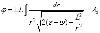 , (42)
where ![]() is proportional to the total energy of the
particle and at infinity is equal to
is proportional to the total energy of the
particle and at infinity is equal to ![]() ,
,
![]() is the potential of
the gravitational field.
is the potential of
the gravitational field.
If in (40) we neglect
the curvature of space-time, assuming ![]() ,
eliminating the small terms of the form
,
eliminating the small terms of the form ![]() and
and ![]() , and if we
subtract under the root the rest energy of the unit mass, equal to
, and if we
subtract under the root the rest energy of the unit mass, equal to ![]() , then (40)
turns into (42).
, then (40)
turns into (42).
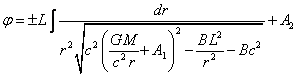
4. Equation of radial motion in GTR
The standard equations of motion of the test particle near the massive body in the GTR was described,
for example, in [18]:
![]() , (43)
, (43)
where ![]() is the proper time of the moving particle as
it determined in GTR.
is the proper time of the moving particle as
it determined in GTR.
Since the interval can
be expressed through the differential of the proper time of the test particle
in the form ![]() , then (16)
can be written as follows:
, then (16)
can be written as follows:
![]() . (44)
. (44)
The non-zero Christoffel
symbols for the spherical coordinates are:
![]() ,
, ![]() ,
, ![]() ,
, ![]() ,
, ![]() ,
,
![]() ,
, ![]() ,
, ![]() .
.
(45)
With ![]() in (43) and metric tensor (1) in (45) only two
Christoffel symbols are nonzero:
in (43) and metric tensor (1) in (45) only two
Christoffel symbols are nonzero: ![]() . Using
. Using ![]() and
and ![]() , taking
into account the definition
, taking
into account the definition ![]() and multiplying (43) by
and multiplying (43) by ![]() , we find:
, we find:
![]() ,
, ![]() ,
, ![]() ,
(46)
,
(46)
where ![]() is some constant, which can be conveniently
associated with the initial velocity at infinity. Indeed, at infinity
is some constant, which can be conveniently
associated with the initial velocity at infinity. Indeed, at infinity
![]() , and the
coordinate time
, and the
coordinate time ![]() is the time of the inertial reference frame in
which the particle is moving at the constant velocity
is the time of the inertial reference frame in
which the particle is moving at the constant velocity ![]() . Then,
according to the special theory of relativity,
. Then,
according to the special theory of relativity, ![]() and
and ![]() .
.
For the motion of the
particle along the radius the angular coordinates ![]() and
and ![]() do not change, and
do not change, and ![]() . In this case,
from (44) for the coordinates
. In this case,
from (44) for the coordinates ![]() and
and ![]() taking into account (1) and
taking into account (1) and ![]() from (46) we obtain:
from (46) we obtain:
![]() .
.
According to the
Schwarzschild metric ![]() , so with
, so with ![]() for radial motion we have:
for radial motion we have:
 . (47)
In a more general case, converting
from spherical coordinates to Cartesian coordinates and then to polar
coordinates, as in the previous section, (43) can be reduced to the following
form:
![]() . (48)
. (48)
 ,
,  .
.
These equations are used
in GTR to describe the planar motion of the bodies relative to the fixed center
in the polar coordinates.
5. Pioneer anomaly
5.1. Qualitative approach
We shall assume that the
spacecraft moves away from Earth and the Sun almost radially, transmitting to
the tracking station the radio signal of known frequency ![]() . Because
of the Doppler effect, the frequency received on Earth
will change to:
. Because
of the Doppler effect, the frequency received on Earth
will change to:
 , (49)
where ![]() is the velocity of the spacecraft relative to
the Earth,
is the velocity of the spacecraft relative to
the Earth,
![]() is the angle between
the velocity and the direction to the radiation detector.
is the angle between
the velocity and the direction to the radiation detector.
As the spacecraft gets
farther from the Sun with turned-off engines, under the influence of solar
attraction the velocity ![]() gradually decreases, so that the frequency
gradually decreases, so that the frequency ![]() should increase. From (49) we can obtain the
change of the velocity of the spacecraft and the relative change of the
frequency during the time
should increase. From (49) we can obtain the
change of the velocity of the spacecraft and the relative change of the
frequency during the time ![]() in which the signal goes from the spacecraft
to the Earth:
in which the signal goes from the spacecraft
to the Earth:
![]() ,
(50)
,
(50)
where ![]() is the total acceleration of the spacecraft.
is the total acceleration of the spacecraft.
The acceleration ![]() is negative, mostly caused by the Sun and
directed towards the Sun, and the velocity
is negative, mostly caused by the Sun and
directed towards the Sun, and the velocity ![]() is directed at the angle
is directed at the angle ![]() away from the direction from the spacecraft to the Sun. We shall further
assume that the relative change in the frequency of the signal (50) is of such
kind that it takes into account all the possible sources of acceleration and
the factors influencing the result. Then the residual signal, which is not
simulated by anything, can also be represented by (50), in which in the place
of acceleration the anomalous acceleration
away from the direction from the spacecraft to the Sun. We shall further
assume that the relative change in the frequency of the signal (50) is of such
kind that it takes into account all the possible sources of acceleration and
the factors influencing the result. Then the residual signal, which is not
simulated by anything, can also be represented by (50), in which in the place
of acceleration the anomalous acceleration ![]() stands:
stands:
 .
(51)
.
(51)
We can estimate the
velocity of the spacecraft depending on the radial distance ![]() from the equation of its free radial motion in
classical mechanics:
from the equation of its free radial motion in
classical mechanics:
![]() , (52)
, (52)
where ![]() is the Sun's mass.
is the Sun's mass.
Assuming in the first
approximation that the motion of the spacecraft is purely radial, we shall
integrate: ![]() . We shall
assume the velocity of the spacecraft at the distance of 87 a.u.
was 12.2 km/s, from this we find
. We shall
assume the velocity of the spacecraft at the distance of 87 a.u.
was 12.2 km/s, from this we find ![]() m2/c2. Consequently, at
the distance
m2/c2. Consequently, at
the distance ![]() a.u. for the
velocity of the spacecraft in the approximation of the free radial motion we
should assume about 14.7 km/s.
a.u. for the
velocity of the spacecraft in the approximation of the free radial motion we
should assume about 14.7 km/s.
We can explain the velocities
of the Pioneers in the following way. From (35) in the approximation of the
radial motion, when the density of the angular momentum ![]() , and with
, and with ![]() , for the
radial velocity of a freely flying spacecraft in CTG we can write:
, for the
radial velocity of a freely flying spacecraft in CTG we can write:
 . (53)
If we proceed from (52),
at the distance of 1 a.u. we can assume that the
initial velocity is equal to ![]() m/s. This allows us to estimate in (53) the
value of the constant
m/s. This allows us to estimate in (53) the
value of the constant ![]() and to find the velocity of the spacecraft at
different distances.
and to find the velocity of the spacecraft at
different distances.
In GTR we have a similar
formula according to (47):
 . (54)
Substituting in (54) ![]() m/s with
m/s with ![]() a.u., we find
a.u., we find ![]() . With the
help of (53) and (54) we calculate the velocity of the spacecraft according to
CTG and GTR at different distances for the case of conditionally radial motion.
The results are shown in Table 1.
. With the
help of (53) and (54) we calculate the velocity of the spacecraft according to
CTG and GTR at different distances for the case of conditionally radial motion.
The results are shown in Table 1.
As we can see, the
velocities of the spacecraft in GTR and CTG are slightly different. If the
spacecraft starts with ![]() a.u., then the time
of its motion up to
a.u., then the time
of its motion up to ![]() a.u. is of the order
of
a.u. is of the order
of ![]() s (this approximate value is obtained by
dividing the distance traveled by the average velocity). During this time up to
the position with
s (this approximate value is obtained by
dividing the distance traveled by the average velocity). During this time up to
the position with ![]() a.u. because
of the different velocities the difference between the positions of the
spacecrafts according to the equations of GTR and CTG will grow up to
a.u. because
of the different velocities the difference between the positions of the
spacecrafts according to the equations of GTR and CTG will grow up to ![]() m. For the spacecraft to move from 5 to 10 a.u. the time required is, accordingly, about
m. For the spacecraft to move from 5 to 10 a.u. the time required is, accordingly, about ![]() s, what is shown in Table 1.
s, what is shown in Table 1.
Table 1. The data on the motion of the spacecraft
|
|
|
|
|
|
|
1 |
4.361 |
|
|
|
|
5 |
2.196624147 CTG 2.196620538
GTR |
3.29 |
1.82 |
19.8 |
|
10 |
1.746714927 CTG 1.746712488 GTR |
13.2 |
3.79 |
18.3 |
|
15 |
1.568321059 CTG 1.568319299 GTR |
9.47 |
4.51 |
9.31 |
|
20 |
1.471033615 CTG 1.471032248 GTR |
7.69 |
4.92 |
6.4 |
Because the velocity of
the spacecraft in CTG is somewhat greater than in GTR, then in case of the measurements
according to the Doppler effect at each time point the
spacecraft is located farther than it is assumed according to GTR. Because of
this difference in the distances the velocity of the spacecraft, always
decreasing with time because of the attraction of the Sun, is less than the
velocity of the spacecraft according to GTR. For example, at the distance ![]() = 5 а.е. + 3.29·105 m according to CTG the
velocity of the spacecraft in our model calculations will be 2.196478495·104
m/s, whereas according to GTR the spacecraft is at the distance of 5 a.u. and has the velocity 2.196620538·104 m/s.
As a result, with the help of the Doppler effect, the
velocity of the spacecraft is registered, decreased relative to the data of
GTR. This decrease is attributed to the anomalous acceleration acting in the
direction towards the Sun.
= 5 а.е. + 3.29·105 m according to CTG the
velocity of the spacecraft in our model calculations will be 2.196478495·104
m/s, whereas according to GTR the spacecraft is at the distance of 5 a.u. and has the velocity 2.196620538·104 m/s.
As a result, with the help of the Doppler effect, the
velocity of the spacecraft is registered, decreased relative to the data of
GTR. This decrease is attributed to the anomalous acceleration acting in the
direction towards the Sun.
In the last column of
Table 1, we estimated the anomalous acceleration by the formula: ![]() . This acceleration indicates that the spacecraft is situated at the
distance that seems to be smaller than expected by the value
. This acceleration indicates that the spacecraft is situated at the
distance that seems to be smaller than expected by the value ![]() , which
arises during the time
, which
arises during the time ![]() because of the difference in velocities. The distances
because of the difference in velocities. The distances ![]() in Table 1 are calculated by an average
velocity at each interval of motion, so to obtain the total result we should
add up all
in Table 1 are calculated by an average
velocity at each interval of motion, so to obtain the total result we should
add up all ![]() . This will
lead over time to the increase in distance between the positions of the
spacecrafts according to GTR and CTG, and to decrease of the anomalous
acceleration
. This will
lead over time to the increase in distance between the positions of the
spacecrafts according to GTR and CTG, and to decrease of the anomalous
acceleration ![]() with the distance as compared with the data in
Table 1. As is shown in Table 1, the values of the anomalous acceleration are
close enough to the data obtained for the effect of Pioneers, and at small
distances up to 5–10 a.u. they are masked by the
acceleration from the pressure force of the solar wind.
with the distance as compared with the data in
Table 1. As is shown in Table 1, the values of the anomalous acceleration are
close enough to the data obtained for the effect of Pioneers, and at small
distances up to 5–10 a.u. they are masked by the
acceleration from the pressure force of the solar wind.
5.2. Analytical approach
Now let us try to derive
the corresponding formula for the anomalous acceleration, again for the case of
purely radial motion. Assuming in (35) ![]() , for the
velocity of the spacecraft in CTG and for its current position relative to the
Sun we obtain:
, for the
velocity of the spacecraft in CTG and for its current position relative to the
Sun we obtain:
 , (55)

(56)
where ![]() is the time component of the metric in CTG, , where
is the time component of the metric in CTG, , where ![]() is the velocity of the spacecraft at infinity,
the radial coordinate
is the velocity of the spacecraft at infinity,
the radial coordinate ![]() is the function of the time
is the function of the time ![]() of the motion from the Sun, and the constant
of the motion from the Sun, and the constant ![]() is the parameter of integration.
is the parameter of integration.
If at a given time point
![]() we know the radial distance
we know the radial distance ![]() and the velocity
and the velocity ![]() , it allows
us to calculate the constants
, it allows
us to calculate the constants ![]() and
and ![]() in (55) and (56). Thus, in the previous
section, we assumed for simplicity that
in (55) and (56). Thus, in the previous
section, we assumed for simplicity that ![]() , at
, at ![]() the spacecraft was at a distance
the spacecraft was at a distance ![]() a.u., and the constant
a.u., and the constant ![]() . These data
can be used to estimate the constant
. These data
can be used to estimate the constant ![]() in (56).
in (56).
We will integrate now
(54) for the radial motion in GTR:
 (57)
(57)
In (57) the constant ![]() appears, which must be found together with the
constant
appears, which must be found together with the
constant ![]() from the initial conditions of motion.
from the initial conditions of motion.
We suppose now that we
have derived from (56) the dependence of the radial distance in CTG as the
function of time: ![]() . Similarly,
from (57) we can determine the dependence of the radial distance in GTR as the
function of time:
. Similarly,
from (57) we can determine the dependence of the radial distance in GTR as the
function of time: ![]() . At a first
approximation, the gravitational acceleration of the Sun depends on the radial
distance according to Newton’s formula, and we can write for the accelerations
in CTG and GTR the following:
. At a first
approximation, the gravitational acceleration of the Sun depends on the radial
distance according to Newton’s formula, and we can write for the accelerations
in CTG and GTR the following:
![]() ,
, ![]() .
.
The anomalous
acceleration as a function of the time of the spacecraft’s radial motion is
found as the difference between these accelerations:
![]() .
.
The meaning of this
equality is that in the case of the Pioneers the acceleration
![]() , calculated
in GTR, is overestimated in the absolute value as compared to the measured
acceleration. If the acceleration
, calculated
in GTR, is overestimated in the absolute value as compared to the measured
acceleration. If the acceleration ![]() in CTG describes the motion more precisely and
is equal to the measured acceleration, then to obtain it
we should subtract the anomalous acceleration from the acceleration in GTR:
in CTG describes the motion more precisely and
is equal to the measured acceleration, then to obtain it
we should subtract the anomalous acceleration from the acceleration in GTR:![]() .
.
6. Conclusion
In GTR the gravitational
field is the same as the metric field with its metric tensor. As a result the
gravitational field does not create the metric similar to electromagnetic field
in equation for the metric, and the metric tensor is calibrated with the help
of Newton's law of universal gravitation. We can suppose that such calibration
is not accurate because Newton's law has no relativistic corrections. On the
other hand in CTG the gravitational field is a fundamental field that has its
stress-energy tensor and can influence the metric in the equation for the
metric. The metric component ![]() in CTG depends on the energy of the gravitational
field and it seems it is more precise then
in CTG depends on the energy of the gravitational
field and it seems it is more precise then ![]() in GTR. The metric component
in GTR. The metric component ![]() is in both equations of motion in CTG and GTR
but the equations are different.
is in both equations of motion in CTG and GTR
but the equations are different.
From the point of view
of CTG the effect of the Pioneers is explained as the result of using an equation
of motion that does not coincide with the equation of motion of GTR.
All computer
calculations associated with the motion of the spacecrafts obligatorily use GTR
and take into account not only the influence of the Sun, but of other planets.
If the equation of motion of CTG is valid, there is no anomalous acceleration in
the effect of Pioneer, and the effect is due to the use of GTR instead of CTG.
The following fact also points out to the probable inaccuracy of GTR that in
the signal from the Pioneers we could see not simulated periodic changes
associated with the diurnal rotation of the Earth and its annual revolution
around the Sun. From Table 1 it follows also that the velocities of the
spacecraft in GTR and CTG at equal distances can differ by several centimetres per second. At the same time, in several
articles the so-called flyby effect has been described, when the velocity of
spacecrafts differs from the calculated values up to several centimetres per second [19-20].
There are also works
such as [21] – [23], according to which the motion of the comets: Halley’s
comet, Encke and others, after their passing near the
planets disturbances of unknown nature are discovered, which are not taken into
account by GTR equations (48). We can assume that the recalculation of the
motion of spacecrafts and comets in terms of CTG with the help of equations (35), (36), and (40) will improve the situation.
References
1. J.D. Anderson,
P.A. Laing, E.L. Lau, A.S. Liu, M.M. Nieto and S.G. Turyshev.
Phys. Rev. D 65, 082004 (2002). doi:10.1103/PhysRevD.65.082004.
2. S.G.
Turyshev, V.T. Toth, G. Kinsella, Siu-Chun Lee, S.M. Lok, and J. Ellis. Phys. Rev. Lett.
108, 241101 (2012). doi:10.1103/PhysRevLett.108.241101.
3. D. Modenini and P. Tortora. Phys.
Rev. D 90, 022004 (2014). doi:10.1103/PhysRevD.90.022004.
4. G.U.
Varieschi. Phys. Res. Int. 2012, 469095
(2012). doi:10.1155/2012/469095.
5. A.F.
Rañada and A. Tiemblo. Can.
J. Phys. 90, 931 (2012). doi:10.1139/p2012-086.
6. M.W.
Kalinowski. CEAS Space J. 5, 19 (2013). doi:10.1007/s12567-013-0042-9.
7. J.D.
Anderson and J.R. Morris. Phys. Rev. D 86, 064023 (2012). doi:10.1103/PhysRevD.86.064023.
8. G.S.M.
Moore and R.E.M. Moore. Astrophys. Space. Sci. 347,
235 (2013). doi:10.1007/s10509-013-1514-2.
9. P.C.
Ferreira. Adv. Space Res. 51, 1266 (2013). doi:10.1016/j.asr.2012.11.004.
10.
M.R. Feldman. PLoS
ONE. 8, e78114 (2013). doi:10.1371/journal.pone.0078114.
11.
S.G. Fedosin. Fizicheskie
teorii i beskonechnaia vlozhennost’ materii. Perm. 2009.
12.
S.G. Fedosin. Int. Front. Sci. Lett. 1, 48 (2014).
13.
W. Pauli. Theory of Relativity. Dover
Publications, New York. 1981.
14.
S.G. Fedosin. Adv. Nat. Sci. 5,
55 (2012). doi:10.3968%2Fj.ans.1715787020120504.2023.
15.
S.G. Fedosin. Int. J. Thermo. 18,
13 (2015). doi:10.5541/ijot.34003.
16.
S.G. Fedosin. The concept of the general force vector
field. vixra.org, 28 June 2014. http://vixra.org/abs/1406.0173.
17.
L.D. Landau and E.M. Lifshitz.
Mechanics, Vol. 1, 3th ed. Butterworth–Heinemann, Oxford, 1976.
18.
L.D. Landau and E.M. Lifshitz.
The Classical Theory of Fields, Vol. 2, 4th ed. Butterworth-Heinemann, Oxford, 1975.
19.
J.D. Anderson and J.G. Williams. Class. Quantum Gravity. 18, 2447 (2001). doi:10.1088/0264-9381/18/13/307.
20.
J.D. Anderson, J.K. Campbell and M.M. Nieto. New Astron. 12, 383 (2007). doi:10.1016/j.newast.2006.11.004.
21.
F.L. Whipple. Astrophys.
J. 111, 375 (1950). doi:10.1086/145272.
22.
B.G. Marsden. Planet. Space Sci. 57, 1098
(2009). doi:10.1016/j.pss.2008.12.007.
23.
T. Kiang. Mon. Not. R. Astron. Soc. 162,
271. (1973). doi:10.1093/mnras/162.3.271.
Source:
http://sergf.ru/apen.htm