Journal of Fundamental and Applied Sciences, Vol. 9, No. 1, pp. 411-467 (2017). http://dx.doi.org/10.4314/jfas.v9i1.25
The substantial
model of the photon
Sergey
G. Fedosin
Sviazeva Str.
22-79, Perm 614088, Perm Krai, Russia
e-mail intelli@list.ru
It is shown that the angular frequency
of the photon is nothing else than the averaged angular frequency of revolution
of the electron cloud’s center during emission and quantum transition between
two energy levels in an atom. On assumption that the photon consists of charged
particles of the vacuum field (of praons), the substantial model of a photon is
constructed. Praons move inside the photon in the same way as they must move in
the electromagnetic field of the emitting electron, while internal periodic
wave structure is formed inside the photon. The properties of praons, including
their mass, charge and speed, are derived in the framework of the theory of
infinite nesting of matter. At the same time, praons are part of nucleons and
leptons just as nucleons are the basis of neutron stars and the matter of
ordinary stars and planets. With the help of the Lorentz transformations, which
correlate the laboratory reference frame and the reference frame, co-moving
with the praons inside the photon, transformation of the electromagnetic field
components is performed. This allows us to calculate the longitudinal magnetic
field and magnetic dipole moment of the photon, and to understand the relation
between the transverse components of the electric and magnetic fields,
connected by a coefficient in the form of the speed of light. The total rest
mass of the particles making up the photon is found, it turns out to be
inversely proportional to the nuclear charge number of the hydrogen-like atom,
which emits the photon. In the presented picture the photon composed of praons
moves at a speed less than the speed of light, and it loses the right to be
called an elementary particle due to its complex structure.
Keywords: matter waves; quantum gravity;
electromagnetic interaction; magnetic moments; properties of photon.
PACS: 03.65.-w, 11, 12.10.Dm, 42.25.-p
1. Introduction
As is known, the more
elementary the particle is, the less we know about it. The photon, the concept
of which appeared more than a hundred years ago in the writings of Albert
Einstein, is not an exception. What seems surprising about this particle is the
absence of the rest mass, but at the same time the presence of wave and
corpuscle properties, high stability and the ability to travel over cosmic
distances with low energy losses, the indissoluble connection between photons
and charged particles in the processes of absorption and emission.
One of the modern methods of
studying the photon structure is experiments on colliding photons with each
other, with protons and electrons. These experiments show that at small
distances a photon can be modelled in the form of fluxes of quarks and gluons
[1]. These fluxes should participate in interactions as is prescribed in
quantum electrodynamics.
In the oscillating model [2] a
photon is regarded as an object periodically changing its volume, the speed of
which is less than the speed of light. In this model, it is assumed that the
rest mass of the photon with the greatest wavelength can be related to the
initial conditions of the early Universe. Based on this assumption the estimate
of the mass of the photon’s inner part is made: ![]() kg.
In contrast, in [3] it is considered that a photon has no proper mass, however
under the influence of the vacuum field the effective mass appears.
kg.
In contrast, in [3] it is considered that a photon has no proper mass, however
under the influence of the vacuum field the effective mass appears.
In [4] the photon diameter is
deemed equal to the wavelength ![]() on the ground that this dimension is the limit
for the wave diffraction. The soliton model of the photon is constructed in
[5], where the equation for the vector potential is used, which is similar to
the generalized Schrödinger equation. In [6] it is indicated that the drawback
of the soliton model is the difficulty to explain the origin of the soliton,
which usually requires a nonlinear medium. The photon diameter according to [7]
is equal to
on the ground that this dimension is the limit
for the wave diffraction. The soliton model of the photon is constructed in
[5], where the equation for the vector potential is used, which is similar to
the generalized Schrödinger equation. In [6] it is indicated that the drawback
of the soliton model is the difficulty to explain the origin of the soliton,
which usually requires a nonlinear medium. The photon diameter according to [7]
is equal to ![]() , and
outside of the photon its field strength must decrease in inverse proportion to
the distance to the photon’s axis. This allows the photon to undergo
interference in the Young's interference experiment. Description of a photon as
a rotating particle in the framework of quantum electrodynamics is presented in
[8].
, and
outside of the photon its field strength must decrease in inverse proportion to
the distance to the photon’s axis. This allows the photon to undergo
interference in the Young's interference experiment. Description of a photon as
a rotating particle in the framework of quantum electrodynamics is presented in
[8].
Due to the lack of key
information about the internal parameters of electromagnetic quanta, the
existing models still require further development and specification, because
they do not allow us to define concretely the actual structure of a photon, to
relate it to the source of emission at the atomic level and to the experimental
data. The purpose of this article is to fill this gap and to provide a more
detailed and well-grounded substantial model of the photon. We will do it based
on the theory of infinite nesting of matter and the substantial model of the
electron [9].
We will start with considering
the basic conditions of emission from a hydrogen-like atom and estimating the
duration of emission, which is necessary to determine the photon’s length in
space and then to calculate its energy density. In Section 3, we will present
the main components of the electric and magnetic fields that are created by the
charge rotating around the nucleus in the near and wave zones. The energy flux
of these fields leads to a standard formula for the charge emission. Our goal
is to use certain electromagnetic field components of the rotating charge to
find the equations of motion for the smallest charged particles of the vacuum
field in Section 4. We consider these particles, called praons, as construction
material not only for photons but also for any other elementary particles,
including nucleons and leptons. Praons have mass and we use the Lorentz factor
to describe their motion at relativistic velocities. This allows us to turn
with the help of Lorentz transformations to the reference frame, co-moving with
praons, and to understand their motion from the standpoint of a fixed photon.
In Section 5, based on the
motion of praons in the electromagnetic field of the emitting electron,
periodically changing in space and time, we construct the substantial model of
the photon. Section 6 concerns the structure of the electromagnetic field and the
strong gravitational field inside the photon and their interaction with praons,
which ensures the photon’s stability. In Sections 7, 8, 9 we derive the Lorentz
factor for praons and the energy fluxes within the photon, the magnetic dipole
moment, and the rest mass of the particles that make up the photon,
respectively.
2. Emission of a photon from a
hydrogen-like atom
According to the Bohr
relation, the energy of a photon as an electromagnetic quantum, emitted during
the electron’s transition from some energy level ![]() to a lower level
to a lower level ![]() , equals the
difference between the total energies of the electron at these levels:
, equals the
difference between the total energies of the electron at these levels:
![]() ,
(1)
,
(1)
here ![]() is the Dirac constant,
is the Dirac constant,
![]() is the angular frequency of the photon.
is the angular frequency of the photon.
But how could we describe more
clearly what is happening in the atom during emission of the quantum? For
simplicity, let us assume that one electron is located in the central-type
field of the hydrogen-like atom. If the electron matter rotates totally
symmetrically relative to the nucleus, then the electron would not emit. This
is due to the fact that for each charge element of the electron matter in an
axisymmetric configuration there is a similar charge element on the opposite
side of the axis, which is moving in the opposite direction. At large
distances, the contribution of the nucleus and of these charge elements into
the total electric field strength ![]() and the magnetic induction
and the magnetic induction ![]() will be compensated, and the resulting energy
flux will be close to zero.
will be compensated, and the resulting energy
flux will be close to zero.
Therefore, in order to produce
emission the electron must move so that its center of inertia is sufficiently
removed from the nucleus. Let us assume that the center of the electron cloud
rotates at a distance ![]() from the nucleus and is held in relative
equilibrium by a force directed towards the nucleus. If the velocity of the
cloud’s center is equal to
from the nucleus and is held in relative
equilibrium by a force directed towards the nucleus. If the velocity of the
cloud’s center is equal to ![]() , then for
the equality of the central and centripetal forces we can write:
, then for
the equality of the central and centripetal forces we can write:
![]() ,
, ![]() , (2)
, (2)
where ![]() is the number of protons in the nucleus,
is the number of protons in the nucleus, ![]() is the elementary charge,
is the elementary charge, ![]() is the vacuum permittivity,
is the vacuum permittivity, ![]() is the electron mass, so that
is the electron mass, so that ![]() is the electric force between the positively charged nucleus with the charge
is the electric force between the positively charged nucleus with the charge ![]() and the negatively charged electron.
and the negatively charged electron.
In (2) we used the
approximately equal symbol, since in case of emission the distance ![]() will slowly decrease and the velocity will
increase. Besides, we do not take into account the change in the intrinsic
electromagnetic energy of the cloud due to the change in the radius and volume
of the cloud as it approaches the nucleus. Then we use the standard formula for
the power of the total electromagnetic emission from the elementary charge,
rotating around a certain center [10]. If we consider the emitted energy per
time
will slowly decrease and the velocity will
increase. Besides, we do not take into account the change in the intrinsic
electromagnetic energy of the cloud due to the change in the radius and volume
of the cloud as it approaches the nucleus. Then we use the standard formula for
the power of the total electromagnetic emission from the elementary charge,
rotating around a certain center [10]. If we consider the emitted energy per
time ![]() up to the sign equal to the change in the
total energy
up to the sign equal to the change in the
total energy ![]() of the electron cloud, then we can write:
of the electron cloud, then we can write:
![]() ,
(3)
,
(3)
here ![]() is the speed of light, and a small coefficient
is the speed of light, and a small coefficient
![]() reflects the fact that the emission from the
electron cloud as a dimensional figure should differ from the emission from of
the rotating electron as a point.
reflects the fact that the emission from the
electron cloud as a dimensional figure should differ from the emission from of
the rotating electron as a point.
Assuming that ![]() ,
where
,
where ![]() is the angular velocity of
rotation of the electron cloud’s center around the nucleus, from the ratio for
the power
is the angular velocity of
rotation of the electron cloud’s center around the nucleus, from the ratio for
the power ![]() and (3) we will find the magnitude of the
force, decelerating the cloud’s rotation:
and (3) we will find the magnitude of the
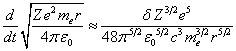
force, decelerating the cloud’s rotation:
![]() .
(4)
.
(4)
For the angular momentum of
the cloud’s center of mass and its rate of change under the influence of the
force moment ![]() we can write:
we can write:
![]() ,
, ![]() . (5)
. (5)
In addition, we obtain the
following:
![]() ,
, ![]() , (6)
, (6)
i.e. the change in the
electron cloud’s energy with the change in the angular momentum of the cloud’s
center is proportional to the angular frequency of rotation.
Expressing from (2) the
rotation speed in the form  and substituting in (5), in view of (4) we
arrive at the differential equation for the dependence of the distance
and substituting in (5), in view of (4) we
arrive at the differential equation for the dependence of the distance ![]() on the time:
on the time:
 ,
, 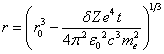 , (7)
, (7)
![]() .
.
here ![]() is the distance to the cloud’s center at the
initial time.
is the distance to the cloud’s center at the
initial time.
Expression (7) approximately
describes the small changes in the distance ![]() over time for the rotational motion of the
electron cloud.
Besides the following condition must hold:
over time for the rotational motion of the
electron cloud.
Besides the following condition must hold: ![]() ,
, ![]() , where
, where ![]() is the time of the cloud’s center of mass
falling onto the attracting center.
is the time of the cloud’s center of mass
falling onto the attracting center.
For example, if we assume that
the distance changes from ![]() to
to ![]() , where
, where ![]() denotes the Bohr radius, then for the time of
transition from the level
denotes the Bohr radius, then for the time of
transition from the level ![]() to the level
to the level ![]() at
at ![]() and
and ![]() from (7) we obtain the value of the order of
from (7) we obtain the value of the order of ![]() s, that is
the typical time of the electromagnetic quantum emission by the electron in
atomic transitions.
s, that is
the typical time of the electromagnetic quantum emission by the electron in
atomic transitions.
If we substitute the distance
(7) in (3), taking into account 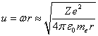 , and
integrate it over the time, we will find the total energy of the electron
cloud:
, and
integrate it over the time, we will find the total energy of the electron
cloud:
![]() .
(8)
.
(8)
From (8) we see that if the
electron moves from the energy level ![]() at the energy level
at the energy level ![]() , then the
energy of the emitted electromagnetic quantum will amount to the value equal to
the difference between the electron’s energy levels in the atom:
, then the
energy of the emitted electromagnetic quantum will amount to the value equal to
the difference between the electron’s energy levels in the atom: ![]() . This
relation fully coincides with the Bohr condition for energies. This should have
been expected, because from (2) it follows that the electrostatic energy of the
electron at the level
. This
relation fully coincides with the Bohr condition for energies. This should have
been expected, because from (2) it follows that the electrostatic energy of the
electron at the level ![]() is equal to the value
is equal to the value ![]() , and the
kinetic energy of the electron is
, and the
kinetic energy of the electron is ![]() . The total
energy at the level
. The total
energy at the level ![]() is supposed to be equal to the sum of these
energies:
is supposed to be equal to the sum of these
energies: ![]() .
.
From the condition 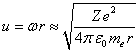 and (3) it follows that the power of the energy
emission is strongly dependent on the current distance
and (3) it follows that the power of the energy
emission is strongly dependent on the current distance ![]() :
:
![]() .
(9)
.
(9)
According to (9) we can assume
that the basic energy of the electromagnetic quantum during the transition from
the energy level ![]() to the energy level
to the energy level ![]() is emitted by the electron cloud near the
level
is emitted by the electron cloud near the
level ![]() , where the
radius of rotation
, where the
radius of rotation ![]() of the electron cloud’s center is less. In
this case, we find explanation for the fact that the frequency of
electromagnetic quanta
of the electron cloud’s center is less. In
this case, we find explanation for the fact that the frequency of
electromagnetic quanta ![]() in (1) is close, but always less than the
frequency of the electron cloud’s rotation near the energy level
in (1) is close, but always less than the
frequency of the electron cloud’s rotation near the energy level ![]() . If we
consider at some time point the emitted electromagnetic quantum along its
length in space, then its oscillation frequency should increase when moving
from the front part of the quantum to its rear part, and the quantum energy
density must reach the maximum closer to the rear part of the quantum.
. If we
consider at some time point the emitted electromagnetic quantum along its
length in space, then its oscillation frequency should increase when moving
from the front part of the quantum to its rear part, and the quantum energy
density must reach the maximum closer to the rear part of the quantum.
The constant ![]() was introduced by Planck in 1900 while
establishing the law of energy distribution in the blackbody spectrum. This
constant turned out to be a universal quantity at the level of elementary
particles and atoms, with the dimensionality of a quantum of action. Its role
in determining the electromagnetic energy of quanta, despite the fact that the
wave oscillation frequency inside these quanta in our opinion cannot be
strictly constant, is quite similar to that of the Boltzmann constant in
determining the average thermal energy of a set of particles through the
temperature, with the energy spread of individual particles, which is always
present.
was introduced by Planck in 1900 while
establishing the law of energy distribution in the blackbody spectrum. This
constant turned out to be a universal quantity at the level of elementary
particles and atoms, with the dimensionality of a quantum of action. Its role
in determining the electromagnetic energy of quanta, despite the fact that the
wave oscillation frequency inside these quanta in our opinion cannot be
strictly constant, is quite similar to that of the Boltzmann constant in
determining the average thermal energy of a set of particles through the
temperature, with the energy spread of individual particles, which is always
present.
We will show that the angular
frequency ![]() of the quantum is the averaged angular frequency
of the quantum is the averaged angular frequency ![]() of rotation of the electron cloud’s center at
transition between the energy levels
of rotation of the electron cloud’s center at
transition between the energy levels ![]() and
and ![]() . For
. For ![]() in view of (6) we have:
in view of (6) we have:
 .
.
At ![]() the energy electromagnetic quantum is:
the energy electromagnetic quantum is:
![]() . (10)
. (10)
From
comparison of (10) and (1) we see that ![]() .
However, if for some reason
.
However, if for some reason ![]() , the
equality
, the
equality ![]() would not exist.
would not exist.
Since during
the emission of quanta the electron’s angular momentum changes, the change in
the angular momentum should be carried away by the electromagnetic quantum.
Photons or electromagnetic quanta, are attributed the angular momentum, equal
to ![]() .
Therefore, during emission the electron loses the angular momentum of the order
of
.
Therefore, during emission the electron loses the angular momentum of the order
of ![]() and the same angular momentum is acquired by
the photon; the electron loses the energy of the order of
and the same angular momentum is acquired by
the photon; the electron loses the energy of the order of ![]() , where
, where ![]() is the average rotation frequency of the
electron’s center of mass near the nucleus for the period of emission, and the
photon acquires this energy. The electron acts in this case as a carrier
particle that transfers its kinetic energy and angular momentum into the energy
and angular momentum of the electromagnetic wave that are concentrated in the
emitted photon.
is the average rotation frequency of the
electron’s center of mass near the nucleus for the period of emission, and the
photon acquires this energy. The electron acts in this case as a carrier
particle that transfers its kinetic energy and angular momentum into the energy
and angular momentum of the electromagnetic wave that are concentrated in the
emitted photon.
3. The emission from the rotating
point charge
Let us assume that a charged
point particle with the charge ![]() rotates by a circle of radius
rotates by a circle of radius ![]() with the angular velocity
with the angular velocity ![]() and the orbital velocity
and the orbital velocity ![]() . We will
place a spherical reference frame at the center of this circle and will seek
for the components of the electromagnetic field strength from the rotating charge
at some remote point with the radius-vector
. We will
place a spherical reference frame at the center of this circle and will seek
for the components of the electromagnetic field strength from the rotating charge
at some remote point with the radius-vector ![]() . The
current position of the charge is given by the vector
. The
current position of the charge is given by the vector ![]() , so that
the circle of rotation lies in the plane
, so that
the circle of rotation lies in the plane ![]() .
.
In order to determine the
electric field strength ![]() and the magnetic field induction
and the magnetic field induction ![]() in the first approximation we will use the
formulas that take into account any motion of the charge in the special theory
of relativity:
in the first approximation we will use the
formulas that take into account any motion of the charge in the special theory
of relativity:
 ,
, ![]() , (11)
, (11)
here ![]() is the vector from the charge to the remote
point at the early time point
is the vector from the charge to the remote
point at the early time point ![]() ,
,
![]() ,
,
![]() is the unit vector, directed from the charge to
the remote point, taken for the case of rotation of this charge by a circle at
an early time point
is the unit vector, directed from the charge to
the remote point, taken for the case of rotation of this charge by a circle at
an early time point ![]() .
.
The formula (11) was first
published by Oliver Heaviside in 1902. It was independently discovered by R. P.
Feynman, in about 1950, and given in some lectures as a good way of thinking
about synchrotron radiation [11].
From the definitions of ![]() and
and ![]() we see that they are mutually dependent. We
will take for them the derivatives with respect to time:
we see that they are mutually dependent. We
will take for them the derivatives with respect to time:
![]() ,
, ![]() ,
,
and then we will express these
derivatives independently from each other:
 ,
,  .
.
If the orbital velocity ![]() is significantly less than the speed of light
is significantly less than the speed of light ![]() , as is the
case for the electron in the atom, we see that:
, as is the
case for the electron in the atom, we see that:
![]() ,
, ![]() . (12)
. (12)
Taking the first time
derivative of the unit vector of the original direction, we find:
![]() , (13)
, (13)
![]() ,
, ![]() .
.
Let us substitute in the
right-hand side of (13) the time derivatives by their maximum values according
to (12) and calculate the second time derivatives of the unit vector:
![]() ,
,
![]() ,
,
![]() .
(14)
.
(14)
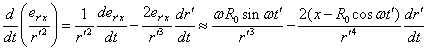
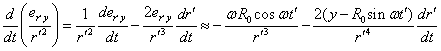
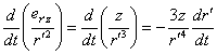
For the components of the
derivative ![]() in (11), in view of (12) and (13), we obtain:
in (11), in view of (12) and (13), we obtain:
 ,
,
 ,
,
 . (15)
Substituting (14) and (15) in
(11), we find the component of the electric field strength ![]() :
:
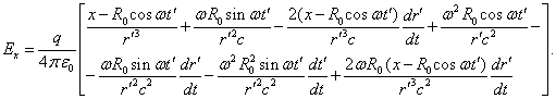 (16)
(16)
According to (12), ![]() , and
then in (16) the third and seventh terms are less than the first term, since
, and
then in (16) the third and seventh terms are less than the first term, since ![]() . Similarly,
taking into account the relation
. Similarly,
taking into account the relation ![]() , the fifth
and sixth terms in (16) are always less than the second term. As a result,
leaving the greatest terms in (16) and (11), for the electromagnetic field
components we have the following:
, the fifth
and sixth terms in (16) are always less than the second term. As a result,
leaving the greatest terms in (16) and (11), for the electromagnetic field
components we have the following:
 .
.
 .
.
![]() . (17)
. (17)
 ,
,  ,
,
 .
.
At large distances, when ![]() , the
last terms containing
, the
last terms containing ![]() in the denominator start predominating in the
electric field components (17), and the terms containing
in the denominator start predominating in the
electric field components (17), and the terms containing ![]() in the denominator start predominating in the
magnetic field components.
in the denominator start predominating in the
magnetic field components.
The Poynting vector or the
electromagnetic energy flux equals:
![]() .
.
If in (17) we take into account only the last terms that remain at a great distance, then the Poynting vector components are as follows:
 ,
,
 ,
,
![]() .
.
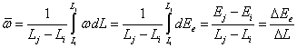
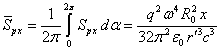
We must first average the
components ![]() and
and ![]() for one period of the charge’s rotation, when
the phase
for one period of the charge’s rotation, when
the phase ![]() varies from 0 to
varies from 0 to ![]() . Given that
. Given that ![]() , we have:
, we have:
 ,
,  .
.
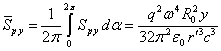
Now, integrating ![]() over the surface of the remote sphere we find
the rate of the electromagnetic energy flux, averaged over the period:
over the surface of the remote sphere we find
the rate of the electromagnetic energy flux, averaged over the period:
![]() . (18)
. (18)
here ![]() is a unit vector perpendicular to the sphere
surface,
is a unit vector perpendicular to the sphere
surface, ![]() is an area unit, for the spherical coordinates
is an area unit, for the spherical coordinates
![]() ,
, ![]() and we assumed that
and we assumed that ![]() .
.
The emission rate in (18)
coincides with the result in (3), while for calculation instead of full expressions
for the field we used only the field components from (17) that remain in the
remote area.
4. Photon formation
4.1. The near zone
We consider an electron in an
atom as a flat disk, the center of which is shifted relative to the nucleus and
is rotating around the nucleus during emission of a photon. After formation, a
photon becomes an independent object and no longer depends on the fields
generated by the emitting electron and the atomic nucleus. Now we need to build
a model of a photon, to understand what it consists of, how it maintains the
perpendicular structure of the electromagnetic field and why a photon is a
stable object. For this purpose, we will turn to the results of [12-13], where
the photon is regarded as an object consisting of tightly bound charged
particles.
In [14] we assume the
positively and negatively charged praons as the charged particles that permeate
entire space in different directions and create the interaction forces between
the electric charges. These particles are one of the components of the vacuum
field, along with the graviton field, responsible for the occurrence of
gravitational forces [15] in Le Sage’s model. The mass to charge ratio found
for praons turns out to be such as it follows from the coefficients of similarity
between different levels of matter and from the theory of dimensions. According
to the theory of infinite nesting of matter, praons make up the matter of
nucleons just as nucleons make up the matter of neutron stars. Besides, the
fluxes of charged praons are the cause of the Coulomb force, and inside of
photons praons come into a state of steady and orderly rotation.
In the substantial model of
electron [9], in a hydrogen atom in its ground state the average radius of the
electron disk is assumed to be equal to the Bohr radius ![]() , the
minimum radius of the disk is
, the
minimum radius of the disk is ![]() and the maximum radius reaches
and the maximum radius reaches ![]() . These
radii correlate with the electron density distribution according to the
electron wave function and the solutions of Schrödinger equation. Close to the
nucleus, at a radius less than
. These
radii correlate with the electron density distribution according to the
electron wave function and the solutions of Schrödinger equation. Close to the
nucleus, at a radius less than ![]() , the
electron matter density decreases rapidly. We suppose that the fluxes of praons
pass here along the axis
, the
electron matter density decreases rapidly. We suppose that the fluxes of praons
pass here along the axis ![]() ,
perpendicular to the plane of the electron disk, without direct contact with
the electron matter, interacting with the nucleus and electron only by means of
the field. From the symmetry of fields of the nucleus and electron disk it
follows that near the axis
,
perpendicular to the plane of the electron disk, without direct contact with
the electron matter, interacting with the nucleus and electron only by means of
the field. From the symmetry of fields of the nucleus and electron disk it
follows that near the axis ![]() the praon fluxes mostly move linearly,
creating the basis of the emitted photon. Other praons that pass through the
electron disk, after interaction with the charged matter of the disk, get into
the photon shell with a cross-section of the order of the electron disk’s size.
The same pattern holds for the hydrogen-like atom.
the praon fluxes mostly move linearly,
creating the basis of the emitted photon. Other praons that pass through the
electron disk, after interaction with the charged matter of the disk, get into
the photon shell with a cross-section of the order of the electron disk’s size.
The same pattern holds for the hydrogen-like atom.
For example, in [14] at a
first approximation a photon is considered as a long, thin cylinder, rotating
at the angular frequency ![]() ,
where
,
where ![]() is the wavelength of the photon. For a photon
with the wavelength
is the wavelength of the photon. For a photon
with the wavelength ![]() m and the angular frequency
m and the angular frequency ![]() s-1, which emerges in the hydrogen
atom at the transition of the electron from the second to the first level in
the Lyman series, we assume the average radius of the electron disk
s-1, which emerges in the hydrogen
atom at the transition of the electron from the second to the first level in
the Lyman series, we assume the average radius of the electron disk ![]() as the photon radius. The total length of the photon is given by the
expression
as the photon radius. The total length of the photon is given by the
expression ![]() , where
, where ![]() is the duration of the photon emission by the
atom, according to (7).
is the duration of the photon emission by the
atom, according to (7).
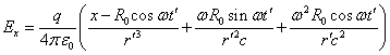
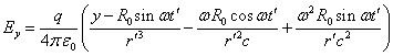
Let us analyze the
electromagnetic field components at an arbitrary point in space ![]() , the
coordinates
, the
coordinates ![]() and
and ![]() of which do not exceed much the orbit radius
of which do not exceed much the orbit radius ![]() of the rotating emitting charge, and the
coordinate
of the rotating emitting charge, and the
coordinate ![]() by its absolute value is much larger than the
orbit radius:
by its absolute value is much larger than the
orbit radius:![]() . In this
area, the condition
. In this
area, the condition ![]() holds, so that in (17) the first terms
predominate. Turning to the hydrogen-like atom, in (17) we will also replace
holds, so that in (17) the first terms
predominate. Turning to the hydrogen-like atom, in (17) we will also replace ![]() with the negative charge of the electron
with the negative charge of the electron ![]() , where
, where ![]() is the elementary charge, and will add to (17)
the static electric field components from the charge
is the elementary charge, and will add to (17)
the static electric field components from the charge ![]() of the atomic nucleus, located in the center
of the coordinate system. The result for the field components can be written as follows:
of the atomic nucleus, located in the center
of the coordinate system. The result for the field components can be written as follows:
![]() ,
, ![]() ,
, ![]() . (19)
. (19)
![]() ,
, ![]() ,
, ![]() .
.
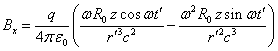
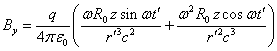
The magnetic field component ![]() in (19) oscillates in a
complicated way. If we restrict ourselves to an area, where
in (19) oscillates in a
complicated way. If we restrict ourselves to an area, where ![]() , that is
outside the atom, but with the near zone condition
, that is
outside the atom, but with the near zone condition ![]() , then we
can assume
, then we
can assume ![]() and
and ![]() . In this
case, the component
. In this
case, the component ![]() can be neglected, since it would be
can be neglected, since it would be ![]() times less than the components
times less than the components ![]() and
and ![]() .
.
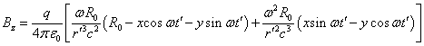
The electric field components,
depending on the multiplier ![]() , determine
the constant field from the effective charge
, determine
the constant field from the effective charge ![]() of the hydrogen-like atom, decreasing with the
distance according to the Coulomb's law. This field should accelerate the
charged praons, changing their energy. However, the emerging photon has the
almost same number of positive and negative praons, which ensures the
electroneutrality of the photon. These praons also interact strongly with each
other and are in a bound state. Then the component
of the hydrogen-like atom, decreasing with the
distance according to the Coulomb's law. This field should accelerate the
charged praons, changing their energy. However, the emerging photon has the
almost same number of positive and negative praons, which ensures the
electroneutrality of the photon. These praons also interact strongly with each
other and are in a bound state. Then the component ![]() at sufficiently large distances
at sufficiently large distances ![]() will not influence the motion of particles in
a neutral average photon.
will not influence the motion of particles in
a neutral average photon.
As a result, the pattern of
the moving field will be formed mainly by those components in ![]() ,
, ![]() ,
, ![]() and
and ![]() that are time-dependent. Introducing the
transverse vectors
that are time-dependent. Introducing the
transverse vectors ![]() and
and ![]() , from (19)
we find for those components the following:
, from (19)
we find for those components the following:
![]() ,
, ![]() , (20)
, (20)
where the unit vector ![]() determines the position of the rotating
electron in the plane
determines the position of the rotating
electron in the plane ![]() at the early time point
at the early time point ![]() .
.
From (20) we see that the
transverse components of the electric ![]() and magnetic
and magnetic ![]() fields rotate around the axis
fields rotate around the axis ![]() at the angular frequency
at the angular frequency ![]() synchronously with the rotation of the vector
synchronously with the rotation of the vector ![]() and with the rotation of the electron in the
atom. At the same time the component
and with the rotation of the electron in the
atom. At the same time the component ![]() is directed in space the same way as the
radius vector of the electron at the early time, and the magnetic field
is directed in space the same way as the
radius vector of the electron at the early time, and the magnetic field ![]() is directed oppositely.
is directed oppositely.
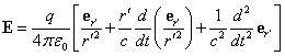
We will write down the
equation of motion of the negatively charged praons in the external
electromagnetic field and will find the mode of their motion, using the general
equations of motion in the same way as in [16-17]. The equation of motion with
respect to the early time ![]() is determined by the Lorentz force:
is determined by the Lorentz force:
![]() , (21)
, (21)
here ![]() is the invariant mass of a negatively charged
praon,
is the invariant mass of a negatively charged
praon,
![]() is the Lorentz factor,
is the Lorentz factor,
![]() is the elementary charge for praon level of
matter,
is the elementary charge for praon level of
matter,
![]() is the particle velocity vector.
is the particle velocity vector.
After substitution of the
fields (20) into (21), we obtain for the motion of particles the following:
![]() ,
,
![]() ,
,
![]() . (22)
. (22)
We will take into account that
the Lorentz force components in (22), containing ![]() in the denominator, can be excluded from calculation because they are
much less than the components without the speed of light. From the ratio of
these components the condition follows:
in the denominator, can be excluded from calculation because they are
much less than the components without the speed of light. From the ratio of
these components the condition follows: ![]() . The
velocity of praons
. The
velocity of praons ![]() along the axis
along the axis ![]() reaches almost the speed of light, so that the
condition has the form
reaches almost the speed of light, so that the
condition has the form ![]() , which
corresponds to the previously accepted expression
, which
corresponds to the previously accepted expression ![]() for the near zone. Consequently, an
approximate solution to the equations (22) for the particles’ velocity has the
form:
for the near zone. Consequently, an
approximate solution to the equations (22) for the particles’ velocity has the
form:
![]() ,
, ![]() ,
, ![]() .
.
What would change, if at these
velocities we will take into account that the electric field components (19)
also contain constant terms, containing the multiplier ![]() ? If
the action of the field component
? If
the action of the field component ![]() can be neglected, then taking into account the
constant terms in the components
can be neglected, then taking into account the
constant terms in the components ![]() and
and ![]() leads to emerging of an additional centripetal
force. This force influences the negative praons and changes their velocity on
the stable rotation trajectory up to the following values:
leads to emerging of an additional centripetal
force. This force influences the negative praons and changes their velocity on
the stable rotation trajectory up to the following values:
![]() ,
, ![]() ,
, ![]() .
.
(23)
For the hydrogen atom ![]() and the expressions for velocities are
simplified. In this case, from (23) we see that in the near zone at the time
and the expressions for velocities are
simplified. In this case, from (23) we see that in the near zone at the time ![]() , which does
not exceed the period of the electron’s rotation around the nucleus, the
negative praons rotate around the axis
, which does
not exceed the period of the electron’s rotation around the nucleus, the
negative praons rotate around the axis ![]() at velocity
at velocity ![]() following the electron’s rotation in the atom. For the positive praons,
at the same angular velocity vector, the linear velocity components in (23)
will be in opposite direction relative to the velocity components of the
negative praons, due to a different sign of charge. For such motion, it is
enough for the negative praons to rotate on the same side as the electron at
the early time and for the positive praons to be on the opposite side relative
to the axis
following the electron’s rotation in the atom. For the positive praons,
at the same angular velocity vector, the linear velocity components in (23)
will be in opposite direction relative to the velocity components of the
negative praons, due to a different sign of charge. For such motion, it is
enough for the negative praons to rotate on the same side as the electron at
the early time and for the positive praons to be on the opposite side relative
to the axis ![]() , at equal
common rotation. We can also take into account that the negative praons at
their matter level are the analogues of electrons and therefore the mass ratio
of positive and negative praons is equal to the mass ratio of proton and
electron:
, at equal
common rotation. We can also take into account that the negative praons at
their matter level are the analogues of electrons and therefore the mass ratio
of positive and negative praons is equal to the mass ratio of proton and
electron: ![]() .
Substituting
.
Substituting ![]() instead of
instead of ![]() in (23) leads to the fact that the velocities and
radii of rotation of the positive praons will be significantly less than those
of the negative praons.
in (23) leads to the fact that the velocities and
radii of rotation of the positive praons will be significantly less than those
of the negative praons.
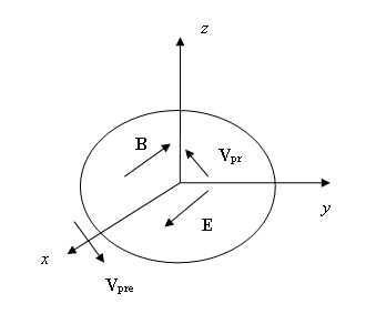
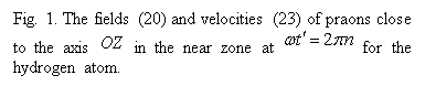
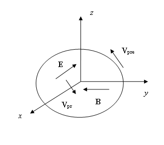
Figure 1 shows a surface
perpendicular to the axis ![]() and shifted along this axis for a certain
distance from the atom, on which we can see the directions of the electric and
magnetic fields (20) and the velocities of praons according to (23) for the
hydrogen atom at
and shifted along this axis for a certain
distance from the atom, on which we can see the directions of the electric and
magnetic fields (20) and the velocities of praons according to (23) for the
hydrogen atom at ![]() . All
vectors correspond to the time point
. All
vectors correspond to the time point ![]() , at which
the condition
, at which
the condition ![]() is met, where
is met, where ![]() . The vector
. The vector
![]() stands for the velocity of the positive
praons.
stands for the velocity of the positive
praons.
4.2. The wave zone
Let us now consider another
extreme case, when the coordinate ![]() is in the remote wave zone. Here the
properties of the emerging photon should reveal themselves to the full extent.
If we consider the electric field strength components in (17), we see that
among all the terms those terms become the maximum terms, which contain the
square of the speed of light. These terms slowly decrease with the distance,
because they contain the distance
is in the remote wave zone. Here the
properties of the emerging photon should reveal themselves to the full extent.
If we consider the electric field strength components in (17), we see that
among all the terms those terms become the maximum terms, which contain the
square of the speed of light. These terms slowly decrease with the distance,
because they contain the distance ![]() to the first power in the denominator. In the
magnetic components, the largest terms also slowly decrease with the distance,
since they are proportional to the multiplier
to the first power in the denominator. In the
magnetic components, the largest terms also slowly decrease with the distance,
since they are proportional to the multiplier ![]() .
.
Turning again to the hydrogen
atom, we will replace ![]() in (17) with the electron’s negative charge
in (17) with the electron’s negative charge ![]() and will add to (17) the components of the
static electric field from the charge
and will add to (17) the components of the
static electric field from the charge ![]() of the atomic nucleus, located in the center
of the coordinate system. As a result, the field components in the wave zone
can be expressed as follows:
of the atomic nucleus, located in the center
of the coordinate system. As a result, the field components in the wave zone
can be expressed as follows:
![]() ,
, ![]() ,
, ![]() .
.
(24)
![]() ,
, ![]() ,
, ![]() .
.
We will consider sufficiently
long distances ![]() ,
when the conditions
,
when the conditions  ,
,  are met. Then in the components
 ![]() and
and ![]() in (24) we can neglect the constant terms from
the nuclear field. As for component
in (24) we can neglect the constant terms from
the nuclear field. As for component ![]() , it should
have little effect on the photon’s motion also due to its electrical
neutrality.
, it should
have little effect on the photon’s motion also due to its electrical
neutrality.
The magnetic field component ![]() as compared with the components
as compared with the components ![]() and
and ![]() is small. For example, the amplitude ratio of
the components
is small. For example, the amplitude ratio of
the components ![]() and
and ![]() at small
at small ![]() and
and ![]() is estimated as
is estimated as ![]() . Further on
we will consider that the component
. Further on
we will consider that the component ![]() is close to zero and in the wave zone it is
not involved in the processes inside the photon. Then the electric and magnetic
fields that remain in (24) would be perpendicular to each other and to the axis
is close to zero and in the wave zone it is
not involved in the processes inside the photon. Then the electric and magnetic
fields that remain in (24) would be perpendicular to each other and to the axis
![]() , besides
the magnetic field components would be shifted forward relative to the electric
field components at an angle
, besides
the magnetic field components would be shifted forward relative to the electric
field components at an angle ![]() and rotate at the same frequency
and rotate at the same frequency ![]() . In
addition, the relation
. In
addition, the relation ![]() appears. In a photon the same conditions are met, and it is expected
that the fields in the form of (24) should form a circularly polarized photon,
that is, with rotation of the electric vector relative to the photon’s axis.
appears. In a photon the same conditions are met, and it is expected
that the fields in the form of (24) should form a circularly polarized photon,
that is, with rotation of the electric vector relative to the photon’s axis.
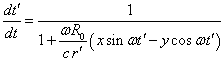
In (24) we will turn from the
earlier time ![]() to the current time
to the current time ![]() in the laboratory reference frame, taking into
account the definition:
in the laboratory reference frame, taking into
account the definition: ![]() . We will
also introduce the wave vector with the amplitude
. We will
also introduce the wave vector with the amplitude ![]() , which is
directed along the axis
, which is
directed along the axis ![]() , so that at
any sign of the coordinate
, so that at
any sign of the coordinate ![]() and velocity of praons
and velocity of praons ![]() the following relations are satisfied:
the following relations are satisfied: ![]() ,
, ![]() . Then
. Then ![]() , and for
periodically varying fields we can write the following:
, and for
periodically varying fields we can write the following:
![]() ,
, ![]() ,
,
![]() ,
, ![]() ,
,
![]() ,
, ![]() . (25)
. (25)
As we can see, at any constant
value ![]() , the
fields in (25) depend on the time according to the sine law. In addition, as
the coordinate
, the
fields in (25) depend on the time according to the sine law. In addition, as
the coordinate ![]() increases at the points, where the condition
increases at the points, where the condition ![]() is satisfied and
is satisfied and ![]() , the fields
(25) rotate synchronously with each other along the axis
, the fields
(25) rotate synchronously with each other along the axis ![]() . Thus, the
field acquires a periodic spatial structure, repeated after a minimum distance
equal to the wavelength. In the previous case, when equation (21) was solved,
the spatial structure was not considered, as we were considering the near zone,
the size of which is of the order of less than one wavelength.
. Thus, the
field acquires a periodic spatial structure, repeated after a minimum distance
equal to the wavelength. In the previous case, when equation (21) was solved,
the spatial structure was not considered, as we were considering the near zone,
the size of which is of the order of less than one wavelength.
Similarly to (21), we will
write the equation of motion for the negative praons, but with respect to the
current time ![]() :
:
![]() .
.
After substituting the fields
(25) into this equation we obtain:
 , (26)
 ,
,
 .
.
In the right side of (26) the
Lorentz force depends on two variables – the time ![]() and the coordinate
and the coordinate ![]() that define the distance to the emitting atom.
Therefore, during the motion of the charged particles in the electromagnetic
field, the acceleration and velocity of the particles also become the functions
of
that define the distance to the emitting atom.
Therefore, during the motion of the charged particles in the electromagnetic
field, the acceleration and velocity of the particles also become the functions
of ![]() and
and ![]() . Due to
this, we presented the time derivatives in the left side of (26) as material
derivatives.
. Due to
this, we presented the time derivatives in the left side of (26) as material
derivatives.
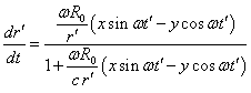
The change of ![]() has a more significant impact on the argument
of sines and cosines than the change of
has a more significant impact on the argument
of sines and cosines than the change of ![]() in the amplitude’s
denominator. If we consider
in the amplitude’s
denominator. If we consider ![]() as a variable only in the sines and cosines,
then the approximate solution of equations (26) for the velocity of the
particles has the form:
as a variable only in the sines and cosines,
then the approximate solution of equations (26) for the velocity of the
particles has the form:
![]() ,
, ![]() ,
, ![]() .
.
(27)
If the time ![]() is fixed, then in case of changing the
position of the coordinate from
is fixed, then in case of changing the
position of the coordinate from ![]() to
to ![]() , the
velocity vector in (27) will make complete revolution around the axis
, the
velocity vector in (27) will make complete revolution around the axis ![]() , while at
large
, while at
large ![]() the decrease of the velocity amplitude due to
the change of
the decrease of the velocity amplitude due to
the change of ![]() will be little. This proves our approximate
solution of (27), though solving the equations we have not taken into account
the change of
will be little. This proves our approximate
solution of (27), though solving the equations we have not taken into account
the change of ![]() in
in ![]() in the denominator of the Lorentz force’s amplitude.
in the denominator of the Lorentz force’s amplitude.
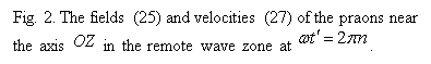
Figure 2 shows a surface
perpendicular to the axis ![]() ,
where the directions of the electric and magnetic fields (25) and praons’
velocities are shown according to (27). The vectors
,
where the directions of the electric and magnetic fields (25) and praons’
velocities are shown according to (27). The vectors ![]() and
and ![]() denote the velocities of the positive and
negative praons, respectively.
denote the velocities of the positive and
negative praons, respectively.
Let us pay attention to the
difference between the solutions (23) and (27), which consists in the fact that
the praons’ velocities in them for the hydrogen atom at ![]() have different signs. In this case, at the boundary between the near and
wave zones, which is reflected by the condition
have different signs. In this case, at the boundary between the near and
wave zones, which is reflected by the condition ![]() , a change
of the field action takes place. Specifically, the total field of the electron
changes its phase to the opposite, due to the increased field components (25)
in comparison with the field components (20). As a result, when the electron is
rotating on the one side from the axis
, a change
of the field action takes place. Specifically, the total field of the electron
changes its phase to the opposite, due to the increased field components (25)
in comparison with the field components (20). As a result, when the electron is
rotating on the one side from the axis ![]() , the
negative praons are located and rotating under the field action on the opposite
side of the axis
, the
negative praons are located and rotating under the field action on the opposite
side of the axis ![]() . As for the
positive praons, they are now located on the side, where the electron is moving,
and are rotating at lower speed and with a smaller radius of rotation, due to
their large mass.
. As for the
positive praons, they are now located on the side, where the electron is moving,
and are rotating at lower speed and with a smaller radius of rotation, due to
their large mass.
Additionally, the photon
obtains spatial structure in the wave zone. How can it be explained from the
standpoint of physics? Assume that the electromagnetic field of the electron,
which is periodically varying in the course of rotation, achieves a certain
cross section of the photon at a distance ![]() from the atom and sets its particles into
motion. Then, the electron makes a revolution inside the atom, and at this
point new particles come to the cross section at
from the atom and sets its particles into
motion. Then, the electron makes a revolution inside the atom, and at this
point new particles come to the cross section at ![]() from the side of the atom. The electron exerts
influence on them by its field, as in the previous case, and everything is
repeated. The same holds true for the points with coordinates
from the side of the atom. The electron exerts
influence on them by its field, as in the previous case, and everything is
repeated. The same holds true for the points with coordinates ![]() , where the
field comes from the electron in the same phase and respectively it was emitted
by the electron at the earlier time points. Since the beginning of the photon’s
emission, as the time was passing and the number of the electron’s revolutions
was increasing, the number of single-phase points with coordinates
, where the
field comes from the electron in the same phase and respectively it was emitted
by the electron at the earlier time points. Since the beginning of the photon’s
emission, as the time was passing and the number of the electron’s revolutions
was increasing, the number of single-phase points with coordinates ![]() was increasing until the rotating field of the electron would not cover
the entire area that should be occupied by the photon. Besides, if the motion
of particles inside the photon occurs in a certain way and synchronously with
the electron’s motion, as in (27), then it creates the necessary conditions for
the wave structure inside the photon, which is periodically varying in space
and time.
was increasing until the rotating field of the electron would not cover
the entire area that should be occupied by the photon. Besides, if the motion
of particles inside the photon occurs in a certain way and synchronously with
the electron’s motion, as in (27), then it creates the necessary conditions for
the wave structure inside the photon, which is periodically varying in space
and time.
The velocity components ![]() in (27) are recorded in the reference frame
in (27) are recorded in the reference frame ![]() , associated
with the atom emitting the photon. Let us now turn to the reference frame
, associated
with the atom emitting the photon. Let us now turn to the reference frame ![]() , which is
moving along the axis
, which is
moving along the axis ![]() at the velocity
at the velocity ![]() almost reaching the speed of light. For this
purpose we will use the direct Lorentz transformations as follows:
almost reaching the speed of light. For this
purpose we will use the direct Lorentz transformations as follows:
 ,
, ![]() ,
, ![]() ,
, ![]() .
.
![]() .
(28)
.
(28)
In ![]() we denoted the proper time with
we denoted the proper time with ![]() , to avoid
confusion with the earlier time
, to avoid
confusion with the earlier time ![]() in (20). We also would need to transform the
velocities, that is to establish relation between the velocities in both
reference frames. In this case, we obtain the following:
in (20). We also would need to transform the
velocities, that is to establish relation between the velocities in both
reference frames. In this case, we obtain the following:
![]() ,
,  ,
, ![]() ,
,
 . (29)
The velocity ![]() denotes the full velocity of the particle in
denotes the full velocity of the particle in ![]() , and
, and ![]() is the Lorentz factor of the particle in
is the Lorentz factor of the particle in ![]() . Let us
substitute into (27) the Lorentz transformation for the wave phase (28) and the
transformation (29) of the velocities and the Lorentz factor, leaving
. Let us
substitute into (27) the Lorentz transformation for the wave phase (28) and the
transformation (29) of the velocities and the Lorentz factor, leaving ![]() in the velocity’s amplitude constant and expressed in terms of the
coordinates in
in the velocity’s amplitude constant and expressed in terms of the
coordinates in ![]() :
:
![]() ,
, ![]() . (30)
. (30)
As is known, the role of the
Lorentz transformations reduces to establishing the relation between the clock
values and the coordinates of events in the inertial reference frames. It
follows from them that in the moving reference frames the rate of clock slows
down. In (30), in the reference frame ![]() , in
view of the relation
, in
view of the relation ![]() and the inverse Lorentz
transformations in the wave phase (28), the role of the angular rate of
rotation of the velocity vector is played by the quantity
and the inverse Lorentz
transformations in the wave phase (28), the role of the angular rate of
rotation of the velocity vector is played by the quantity  . The
angular velocity
. The
angular velocity ![]() is less than the angular velocity of rotation
is less than the angular velocity of rotation ![]() of the electron in the atom and the angular
frequency of the photon due to the time dilation effect. At the same time, in
of the electron in the atom and the angular
frequency of the photon due to the time dilation effect. At the same time, in ![]() the wave vector
the wave vector  becomes smaller and the wavelength
 ![]() becomes larger, which is due
to the effect of reduction of the longitudinal dimensions of the moving bodies
in
becomes larger, which is due
to the effect of reduction of the longitudinal dimensions of the moving bodies
in ![]() .
.
According to (30), in the
reference frame ![]() we observe rotation of the negative praons at
the angular velocity
we observe rotation of the negative praons at
the angular velocity ![]() in the plane
in the plane ![]() , and in
case of instantaneous motion of the observer along the axis
, and in
case of instantaneous motion of the observer along the axis ![]() with changing of
with changing of ![]() we discover displacement of the rotation phase
by the value
we discover displacement of the rotation phase
by the value ![]() . For this
to happen the particles inside the photon must be arranged as if they are
located on the surface of the right-threaded screw with the pitch
. For this
to happen the particles inside the photon must be arranged as if they are
located on the surface of the right-threaded screw with the pitch ![]() , while the
screw is rotating to the right at the angular velocity
, while the
screw is rotating to the right at the angular velocity ![]() , without
moving along the axis
, without
moving along the axis ![]() . If we
consider the positive praons as the rotating particle inside the photon, then
due to their increased mass, their rotation velocity in (30) would be less. The
positive praons can be placed on the surface of the screw, the radius of which
is
. If we
consider the positive praons as the rotating particle inside the photon, then
due to their increased mass, their rotation velocity in (30) would be less. The
positive praons can be placed on the surface of the screw, the radius of which
is ![]() times less than the radius of the screw for
the negative praons. At each time point the positive praons would be on the
same side as the electron at a corresponding delayed time
times less than the radius of the screw for
the negative praons. At each time point the positive praons would be on the
same side as the electron at a corresponding delayed time ![]() , while the
negative praons would be located on the other side of the axis
, while the
negative praons would be located on the other side of the axis ![]() .
.
4.3. The second field component
Let us consider the action of the
second field component in (17) on the motion of the particles inside the photon
in the wave zone. The field of this component at ![]() in view of the electric field of the nucleus
is as follows:
in view of the electric field of the nucleus
is as follows:
![]() ,
, ![]() ,
, ![]() .
.
(31)
![]() ,
, ![]() ,
, ![]() .
.
Under conditions ![]() ,
, ![]() , in the
electric field components in (31) we can neglect the constant terms from the
nuclear field including
, in the
electric field components in (31) we can neglect the constant terms from the
nuclear field including ![]() .
Additionally, we can also neglect the magnetic field component
.
Additionally, we can also neglect the magnetic field component ![]() , since it
would be
, since it
would be ![]() times less than the components
times less than the components ![]() and
and ![]() . In (31)
let us turn from the early time point
. In (31)
let us turn from the early time point ![]() to the current time point
to the current time point ![]() , taking
into account the definition:
, taking
into account the definition: ![]() . At
. At ![]() we find:
we find:
![]() ,
, ![]() ,
,
![]() ,
, ![]() ,
,
![]() ,
, ![]() . (32)
. (32)
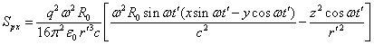
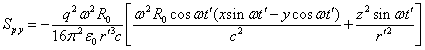
Doing the same as in the
previous section, similarly to (26) we obtain the following:
![]() ,
,
![]() ,
,
![]() .
.
The approximate solution of
these equations for the velocity of particles has the form:
![]() ,
, ![]() ,
, ![]() .
.
(33)
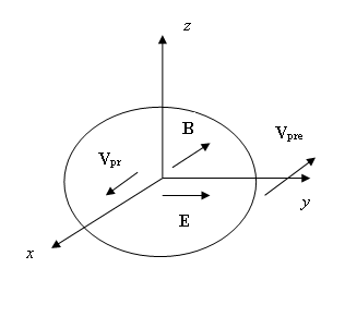
Figure 3 shows the surface
perpendicular to the axis ![]() , on
which the directions of the electric and magnetic fields (32) and the
velocities of praons are shown, according to (33). All the vectors correspond to
the time point
, on
which the directions of the electric and magnetic fields (32) and the
velocities of praons are shown, according to (33). All the vectors correspond to
the time point ![]() , at which
the condition
, at which
the condition ![]() is met. The vectors
is met. The vectors ![]() and
and ![]() denote the velocities of the positive and
negative praons, respectively.
denote the velocities of the positive and
negative praons, respectively.
5. The photon structure
The presence of ![]() in the denominator of the velocity in (23) for
the near zone and in (27) for the wave zone leads to decreasing of the velocity
amplitude while the distance from the emitting atom is increasing. Obviously,
for the photon to exist independently at a certain distance from the atom, the
amplitude of the rotation velocity of the negatively charged praons in the
photon must stop being dependent on
in the denominator of the velocity in (23) for
the near zone and in (27) for the wave zone leads to decreasing of the velocity
amplitude while the distance from the emitting atom is increasing. Obviously,
for the photon to exist independently at a certain distance from the atom, the
amplitude of the rotation velocity of the negatively charged praons in the
photon must stop being dependent on ![]() . By analogy
with (20) and (25), in which we will replace
. By analogy
with (20) and (25), in which we will replace ![]() with a certain constant distance
with a certain constant distance ![]() , we will
assume the following expressions for the amplitude of the electric field inside
the photon in the near zone and in the wave zone, respectively:
, we will
assume the following expressions for the amplitude of the electric field inside
the photon in the near zone and in the wave zone, respectively:
![]() ,
, ![]() .
.
We have an opportunity to
estimate the value of ![]() using the data from [14] for the photon with
the angular frequency
using the data from [14] for the photon with
the angular frequency ![]() s-1, which emerges in the hydrogen atom
in the electron’s transition from the second to the first level in the Lyman
series, setting the photon radius equal to
s-1, which emerges in the hydrogen atom
in the electron’s transition from the second to the first level in the Lyman
series, setting the photon radius equal to ![]() . Based on
the photon energy and its volume, with equality of the density of this energy
and the electromagnetic energy density, we determine the amplitude of the
electric field inside the photon:
. Based on
the photon energy and its volume, with equality of the density of this energy
and the electromagnetic energy density, we determine the amplitude of the
electric field inside the photon: ![]() V/m.
V/m.
If we equate ![]() and
and ![]() , we obtain
, we obtain ![]() , where
, where ![]() is the Bohr radius. However, if we equate
is the Bohr radius. However, if we equate ![]() and
and ![]() , then we
should obtain
, then we
should obtain ![]() . In the
near zone the field
. In the
near zone the field ![]() is substantially smaller than the field
is substantially smaller than the field ![]() , and
therefore, only at a small distance from the nucleus of the order of
, and
therefore, only at a small distance from the nucleus of the order of ![]() , the field
, the field ![]() could set the photon’s praons in motion so
that it could have a field of the order of
could set the photon’s praons in motion so
that it could have a field of the order of ![]() . At the
boundary between the near and wave zones, which is reflected by the condition
. At the
boundary between the near and wave zones, which is reflected by the condition ![]() , the value
, the value ![]() .
Consequently, the internal electromagnetic energy of the photon, associated
with the motion of the charged particles in it, appears in it already in the
near zone. Here, the particles of the emerging photon are influenced by the
electric field (17), consisting of three main components, which get aligned
with each other at
.
Consequently, the internal electromagnetic energy of the photon, associated
with the motion of the charged particles in it, appears in it already in the
near zone. Here, the particles of the emerging photon are influenced by the
electric field (17), consisting of three main components, which get aligned
with each other at ![]() and the value
and the value ![]() .
.
The amplitude of the
transverse electric field of the second component in (17), according to (32),
at ![]() is equal to
is equal to ![]() . From the
equality
. From the
equality ![]() we obtain the estimate:
we obtain the estimate: ![]() , so that in
the near zone the second component in (17) has lower degree of influence on the
particles inside the photon than the first component, but its influence is
stronger than that of the third field component.
, so that in
the near zone the second component in (17) has lower degree of influence on the
particles inside the photon than the first component, but its influence is
stronger than that of the third field component.
Analyzing the field directions
and the velocities of particles in Figures 1-3, resulting from the field
components (17), in a first approximation we can develop the photon model,
which is symmetric in its form. The photon’s cross section at ![]() in this model is presented in Figure 4.
in this model is presented in Figure 4.
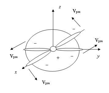
When the rotation phase of the
electron in the atom satisfies the relation ![]() ,
where
,
where ![]() is the earlier time point, then for any time
point
is the earlier time point, then for any time
point ![]() we can choose such
we can choose such ![]() , with which
the pattern of events will be repeated in the same way as in Figure 4. In this
case in Figure 4 the lobes along the axis
, with which
the pattern of events will be repeated in the same way as in Figure 4. In this
case in Figure 4 the lobes along the axis ![]() are formed by the negative praons under action
of the fields of the form (20) and (25), as in Figures 1 and 2, respectively.
In Figure 4, we also added the lobes of the negative praons that are likely to
occur under action of the fields (32), as in Figure 3. In the center, near the
axis
are formed by the negative praons under action
of the fields of the form (20) and (25), as in Figures 1 and 2, respectively.
In Figure 4, we also added the lobes of the negative praons that are likely to
occur under action of the fields (32), as in Figure 3. In the center, near the
axis ![]() the positive praons are concentrated. The
whole lobes’ construction is rotating around the axis
the positive praons are concentrated. The
whole lobes’ construction is rotating around the axis ![]() at the angular velocity
at the angular velocity ![]() and it is also moving along this axis at the
velocity
and it is also moving along this axis at the
velocity ![]() , which is
almost equal to the speed of light. At a given time point
, which is
almost equal to the speed of light. At a given time point ![]() with the change
with the change ![]() the phase
the phase ![]() would change and other lobes would appear in
the new cross section of the photon, which would be shifted relative to the
lobes in Figure 4 at a corresponding angle. This means that the entire set of
lobes of the negative praons form continuous helical lines in space at a pitch
equal to the wavelength and with the length along the axis
would change and other lobes would appear in
the new cross section of the photon, which would be shifted relative to the
lobes in Figure 4 at a corresponding angle. This means that the entire set of
lobes of the negative praons form continuous helical lines in space at a pitch
equal to the wavelength and with the length along the axis ![]() equal to the photon’s length.
equal to the photon’s length.
In this case we can expect that at ![]() formation of the two corresponding lobes stops
and they become independent of the field
formation of the two corresponding lobes stops
and they become independent of the field ![]() , which is decreasing in
amplitude. For the rest of the lobes the same is true at
, which is decreasing in
amplitude. For the rest of the lobes the same is true at ![]() for the field
for the field ![]() and at
and at ![]() for the field
for the field ![]() . Although these estimates are not
entirely accurate, as we assumed the constancy of
. Although these estimates are not
entirely accurate, as we assumed the constancy of ![]() in the denominator of the solutions for the
praons’ velocities (23), (27) and (33), the general result remains the same:
the electric field of the rotating electron cloud is able to create the lobe
structure of the emerging photon. The lobes arising from praons are then fixed
by the forces acting between the praons.
in the denominator of the solutions for the
praons’ velocities (23), (27) and (33), the general result remains the same:
the electric field of the rotating electron cloud is able to create the lobe
structure of the emerging photon. The lobes arising from praons are then fixed
by the forces acting between the praons.
Theoretically, inside each
lobe in Figure 4 there should be sufficiently smooth distribution of the
charge, from the positive charge at the center – to the prevalence of the
negative charge at the edges of the lobes. This should also be accompanied by
smooth change of the mass density along the lobes. In this case, the lobes
contain not only the negative praons but also a significant number of positive
praons. We compare the positive praons with protons and the negative praons
with electrons, and admit the existence of neutral praons as the analogues of
neutrons.
From the solutions for the
velocities of praons (23), (27) and (33) we see that these velocities in a
first approximation do not depend on whether the photon is propagating in the
positive or negative direction of the axis ![]() .
These solutions do not contradict the fact that in quantum transition two
photons will be simultaneously emitted from the atom in opposite directions.
These photons must have oppositely directed circular polarization, that is, have
different rotation directions of the electric vector with respect to the
velocity of the photon.
.
These solutions do not contradict the fact that in quantum transition two
photons will be simultaneously emitted from the atom in opposite directions.
These photons must have oppositely directed circular polarization, that is, have
different rotation directions of the electric vector with respect to the
velocity of the photon.
However, as a rule, except for
the special cases of excitation, a multielectron atom emits one photon. To
explain this, let us turn to the results in [9], where the substantial model of
electron was presented, which was understood not as a charged point, but as a
three-dimensional structure in the form of an electron disk. It is assumed that
the matter in the disk rotates differentially around the disk’s center at the
angular velocity ![]() ,
which depends on the current radius
,
which depends on the current radius ![]() of the matter unit’s location. In addition,
the disk’s center can be located at a distance
of the matter unit’s location. In addition,
the disk’s center can be located at a distance ![]() from the nucleus and rotate around it at the
angular velocity
from the nucleus and rotate around it at the
angular velocity ![]() . The latter
allows us to explain the electron spin as the result of rotation of the
electron disk as a whole around the nucleus, as well as to ensure the possibility
of electromagnetic emission from the atom, while there is rotation at the
angular velocity
. The latter
allows us to explain the electron spin as the result of rotation of the
electron disk as a whole around the nucleus, as well as to ensure the possibility
of electromagnetic emission from the atom, while there is rotation at the
angular velocity ![]() . In [9] we
take into account that the negatively charged matter of the electron cloud is
attracted to the positively charged nucleus and at the same time repels from
itself by electrical forces. In this model, the matter is also under influence
of the strong gravitation from the nucleus with the strong gravitational
constant
. In [9] we
take into account that the negatively charged matter of the electron cloud is
attracted to the positively charged nucleus and at the same time repels from
itself by electrical forces. In this model, the matter is also under influence
of the strong gravitation from the nucleus with the strong gravitational
constant ![]() m3∙kg-1∙s-2.
The sum of all these forces makes the electron matter rotate around the
nucleus. The stable quantized states of the atom’s energy are explained by the
fact that in these states the equality is achieved of the kinetic energy flux
of the electron matter and of the sum of the fluxes of the electromagnetic and
gravitational energies in this matter. Besides, the emission from the atom tends
to zero and the state of the electron disk’s rotation remains unchanged for a
long time and the field momentum is not transferred to the matter.
m3∙kg-1∙s-2.
The sum of all these forces makes the electron matter rotate around the
nucleus. The stable quantized states of the atom’s energy are explained by the
fact that in these states the equality is achieved of the kinetic energy flux
of the electron matter and of the sum of the fluxes of the electromagnetic and
gravitational energies in this matter. Besides, the emission from the atom tends
to zero and the state of the electron disk’s rotation remains unchanged for a
long time and the field momentum is not transferred to the matter.
In the substantial model of
the electron it is important that in the multielectron atom the electron disks are
located in the atomic shells approximately parallel to each other and the
number of electrons in each filled shell is even. This leads to the fact that
the magnetic energy of the atom tends to a minimum, since the magnetic moments
of the respective paired electrons are directed oppositely (the Pauli exclusion
principle). To explain the Pauli principle the well-known Lenz rule is used: as
the magnetic field in the conductor increases, the magnetic field is formed
which opposes the initial magnetic field. If an atom has an unpaired electron
and is combined with a free electron, the latter will have such a rotation of
the disk’s matter as to create a magnetic field, according to the Lenz rule and
to the Pauli principle. This explanation does not require any reference to the
quantum spins of the electrons and is based on the known electromagnetic
phenomena.
For the maximum number of
electrons in the electron shell of the atom there is a quadratic dependence ![]() . As
for the multiplier 2 before
. As
for the multiplier 2 before ![]() , we believe that this is a consequence of the Pauli
principle, as well as of the symmetry in the arrangement of electrons in the
form of rings-disks. As for the quadratic dependence
, we believe that this is a consequence of the Pauli
principle, as well as of the symmetry in the arrangement of electrons in the
form of rings-disks. As for the quadratic dependence ![]() , we can see
that as the shell’s number
, we can see
that as the shell’s number ![]() increases the distance to this shell increases
too. The shell’s area like the sphere’s area varies in proportion to the squared
distance. Therefore, in case of a corresponding change of the distance to the
shell with the number
increases the distance to this shell increases
too. The shell’s area like the sphere’s area varies in proportion to the squared
distance. Therefore, in case of a corresponding change of the distance to the
shell with the number ![]() , the
relative density of electrons as the number of electrons per unit area of the
shell, remains unchanged. Only in this case, the entire matter of each electron
will be located on the shell with the same density, and the total charges and
masses of the electrons on the shells will be integer-valued.
, the
relative density of electrons as the number of electrons per unit area of the
shell, remains unchanged. Only in this case, the entire matter of each electron
will be located on the shell with the same density, and the total charges and
masses of the electrons on the shells will be integer-valued.
Now let us consider the
simplest case, when there are two paired electrons in the form of two parallel
disks, one of them is an excited electron in the state of quantum transition,
the momentum of which decreases with emission of a photon. We see that the situation
for the two opposite fluxes of praons passing through the disk of the excited
electron is asymmetric: one flux of praons passes through the first electron
and then through the second excited electron. The other flux of praons first
passes through the second electron and then through the first electron. Since
the first electron is not excited, the center of its disk is not shifted with
respect to the nucleus and does not rotate, the electron does not emit, and it
influences the flux of praons only by its stationary fields. This results in a
slight shift of the flux of praons, which then interacts with the matter and
fields of the excited electron, and becomes involved in the formation of a
photon in the propagation direction of the flux of praons. The opposite flux of
praons first passes through the disk of the excited electron, and transverse
rotation of praons emerges in this flux, which is necessary for a photon. But
then the flux passes through the disk of the second electron, where the transverse
rotation of praons is suppressed by the action of the electron’s rotating
charged matter, which hinders the formation of a photon in this direction. For
the atomic shell, where the number of electrons is more than two, the situation
gets more complicated, but does not change fundamentally – in order to emit the
photon from the atom mainly in one direction, asymmetry of the excited
electron’s position with respect to other electrons is needed.
6. The fields inside the photon
We should note that the charged
praons themselves cannot generate such an electromagnetic field inside the
photon so that this field in turn could lead to the required motion of
particles and hold them together. For such motion of praons there should either
an additional external force, for example the electromagnetic Lorentz force in
(26) from the field of the rotating electron in the atom, or some internal
non-electromagnetic force. For the praons inside the photon we suppose the
action of strong gravitation [14], which should act between the positively
charged praons in the photon’s core and the negatively charged praons in the
lobes. The other two forces are the electromagnetic force of attraction between
the oppositely charged praons in the photon’s core and in the lobes of the photon
and the electromagnetic force of repulsion of the negative praons from each
other. The praons in the lobes are in the state of continuous rotation, so that
we must also take into account the centripetal force.
Earlier we derived the strong
gravitational constant ![]() for the level of atoms, equating the magnitude
of all the four above-mentioned forces, acting on the electron’s matter in the
hydrogen atom [9], [12]. Let us assume in a first approximation that the same
condition of the forces’ equality holds for the praons inside the photon in the
reference frame
for the level of atoms, equating the magnitude
of all the four above-mentioned forces, acting on the electron’s matter in the
hydrogen atom [9], [12]. Let us assume in a first approximation that the same
condition of the forces’ equality holds for the praons inside the photon in the
reference frame ![]() , associated
with the photon. Let us represent any of the lobes in the form of a capacitor,
one plate of which is positively charged and is located at the axis
, associated
with the photon. Let us represent any of the lobes in the form of a capacitor,
one plate of which is positively charged and is located at the axis ![]() , and the
other plate is negatively charged and is located at the end of lobe. We believe
that the photon is neutral in general and the number of positively and
negatively charged praons in it is equal. The capacitor plates are attracted to
each other by the electric force, as well as by the attraction force of the
strong gravitation:
, and the
other plate is negatively charged and is located at the end of lobe. We believe
that the photon is neutral in general and the number of positively and
negatively charged praons in it is equal. The capacitor plates are attracted to
each other by the electric force, as well as by the attraction force of the
strong gravitation:
![]() ,
, 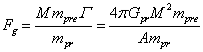 ,
,
where ![]() and
and ![]() are the charge and mass of the positive praons on the capacitor plate,
which is adjacent to the axis
are the charge and mass of the positive praons on the capacitor plate,
which is adjacent to the axis ![]() ; the product
; the product
 is the total mass of the negative praons on
the other capacitor plate at the end of the lobe;
is the total mass of the negative praons on
the other capacitor plate at the end of the lobe; ![]() and
and ![]() set the masses of the positive and negative praons;
set the masses of the positive and negative praons;
![]() and
and ![]() are
the electric filed strength and the gravitational field strength, respectively,
which are acting on the plate with the negative praons,
are
the electric filed strength and the gravitational field strength, respectively,
which are acting on the plate with the negative praons, ![]() denotes the area of the capacitor plate.
denotes the area of the capacitor plate.
From the equality of the forces ![]() and
and ![]() , as well as the condition
, as well as the condition ![]() , we find:
, we find:
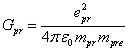 .
(34)
.
(34)
The charge and mass of the
positive praon were found in [14], using the theory of dimensions and the
coefficients of similarity between the atomic and praon levels of matter: ![]() C,
C, ![]() kg, here we
used the coefficients of similarity in mass
kg, here we
used the coefficients of similarity in mass ![]() , in sizes
, in sizes ![]() and in speed of processes
and in speed of processes ![]() .
Substituting the praon’s charge and mass in (34), in view of the relations
.
Substituting the praon’s charge and mass in (34), in view of the relations ![]() ,
, ![]() , we obtain an
estimate of the strong gravitational constant:
, we obtain an
estimate of the strong gravitational constant: ![]() m3·kg-1·s-2.
On the other hand, the gravitational constants at the stellar, atomic and praon
levels of matter, according to the theory of dimensions, are related to each
other by the similarity coefficients:
m3·kg-1·s-2.
On the other hand, the gravitational constants at the stellar, atomic and praon
levels of matter, according to the theory of dimensions, are related to each
other by the similarity coefficients:
![]() m3·kg-1·s-2,
m3·kg-1·s-2, ![]() m3·kg-1·s-2,
m3·kg-1·s-2,
besides, for the strong
gravitational constant at the level of atoms, the following relation from [12]
holds true, which coincides by its sense with (34):
![]() .
.
The strong gravitational constant ![]() allowed us not only to describe the
stability of electrons in the atom, but also to explain the nature of the rest
energy of elementary particles, to derive a formula for the magnetic moment of
the proton [9] and to calculate its radius [18]. The stability of nucleons in
the atomic nucleus is also explained, in this case the strong gravitational
attraction between the nucleons is opposed by the repulsive force of the
torsion fields of the strong gravitation of nucleons (the spin-spin interaction
in the gravitational model of strong interaction). The coupling constant of
strong gravitation is close in value to the standard coupling constant of
strong interaction. In [15] it is shown that the strong gravitation structure
is the same as that of the ordinary gravitation, and the range of the strong
gravitation’s action in the matter, which has the same mass density as that of
the Earth, is not more than 0.7 m [9].
allowed us not only to describe the
stability of electrons in the atom, but also to explain the nature of the rest
energy of elementary particles, to derive a formula for the magnetic moment of
the proton [9] and to calculate its radius [18]. The stability of nucleons in
the atomic nucleus is also explained, in this case the strong gravitational
attraction between the nucleons is opposed by the repulsive force of the
torsion fields of the strong gravitation of nucleons (the spin-spin interaction
in the gravitational model of strong interaction). The coupling constant of
strong gravitation is close in value to the standard coupling constant of
strong interaction. In [15] it is shown that the strong gravitation structure
is the same as that of the ordinary gravitation, and the range of the strong
gravitation’s action in the matter, which has the same mass density as that of
the Earth, is not more than 0.7 m [9].
Thus it can be stated that the
strong gravitation at the level of praons and the electromagnetic forces are
able to keep the positive and negative praons inside the photon near each other
and to ensure the photon’s integrity. As for the stability of the positive
praons concentrated mainly in the photon’s core, here the main forces are the
gravitational forces of attraction and the forces of praons’ repulsion from
each other, according to the gravitational model of strong interaction [9]. In
this model, the gravitational force is opposed by the spin forces from the
gravitational torsion field, which in particular ensures the stability of the
atomic nuclei.
In Figure (4) the electric
field inside the lobes is directed outwardly from the axis ![]() . In
the photon in addition to the electric field there must be a magnetic field
perpendicular to the electric field. In order to understand how this magnetic
field appears, we will consider the rotation of the photon’s lobes in Figure 4
from the perspective of the reference frame
. In
the photon in addition to the electric field there must be a magnetic field
perpendicular to the electric field. In order to understand how this magnetic
field appears, we will consider the rotation of the photon’s lobes in Figure 4
from the perspective of the reference frame ![]() , as in
Section 4.2. This reference frame is moving along the axis
, as in
Section 4.2. This reference frame is moving along the axis ![]() at the same velocity
at the same velocity ![]() as the photon in the reference frame
as the photon in the reference frame ![]() . Taking
into account (29), in
. Taking
into account (29), in ![]() in each cross section of the photon the lobes rotate around the axis
in each cross section of the photon the lobes rotate around the axis ![]() at the angular velocity:
at the angular velocity:
 . (35)
In (35) ![]() denotes the Lorentz factor close to 1 for the
praons in the reference frame
denotes the Lorentz factor close to 1 for the
praons in the reference frame ![]() , and
, and ![]() is a very large Lorentz factor for the praons
in the reference frame
is a very large Lorentz factor for the praons
in the reference frame ![]() , in which
the full velocity
, in which
the full velocity ![]() and the velocity
and the velocity ![]() of the praons are close to the speed of light.
In [14] an estimate of the Lorentz factor for the praons in the photon was
made:
of the praons are close to the speed of light.
In [14] an estimate of the Lorentz factor for the praons in the photon was
made: ![]() . The value
. The value ![]() is substantially less than
is substantially less than ![]() , which
characterizes the effect of time dilation. Inside the lobes a certain electric
field
, which
characterizes the effect of time dilation. Inside the lobes a certain electric
field ![]() is acting, which is in equilibrium with the
strong gravitational field strength and maintains the form of the lobes in view
of their rotation.
is acting, which is in equilibrium with the
strong gravitational field strength and maintains the form of the lobes in view
of their rotation.
Let us consider the
transformation of the electromagnetic field of the lobes from the reference
frame ![]() into the reference frame
into the reference frame ![]() . The
electromagnetic field components are the components of the electromagnetic
field tensor and therefore they can be transformed from one inertial reference
frame into another not as the components of a four-vector, but as the
components of a four-tensor. In particular, for the transformation of the field
components during the motion of the reference frame
. The
electromagnetic field components are the components of the electromagnetic
field tensor and therefore they can be transformed from one inertial reference
frame into another not as the components of a four-vector, but as the
components of a four-tensor. In particular, for the transformation of the field
components during the motion of the reference frame ![]() along the axis
along the axis ![]() we can write:
we can write:
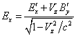 ,
, 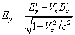 ,
, ![]() , (36)
, (36)
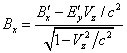 ,
, 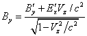 ,
, ![]() .
.
The slow rotation of the
negatively charged lobes creates a certain common magnetic field ![]() . Let
us consider in Figure 4 one of the lobes, in which the internal electric field
at a given time is directed along the axis
. Let
us consider in Figure 4 one of the lobes, in which the internal electric field
at a given time is directed along the axis ![]() and is equal to
and is equal to ![]() . At this
time point, other electric field components averaged with respect to the volume
of the lobe are zero,
. At this
time point, other electric field components averaged with respect to the volume
of the lobe are zero, ![]() and
and ![]() , and
similarly the magnetic field components
, and
similarly the magnetic field components ![]() and
and ![]() . Then from
(36) it follows that for the components of the lobe’s field, which are averaged
with respect to the volume, in the reference frame
. Then from
(36) it follows that for the components of the lobe’s field, which are averaged
with respect to the volume, in the reference frame ![]() we should obtain:
we should obtain:
![]() ,
, ![]() ,
, ![]() ,
, ![]() ,
, 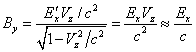 ,
, ![]() .
.
Since ![]() we arrive at the condition
we arrive at the condition ![]() , which
holds in the photon and relates its electric field strength and magnetic field.
Meanwhile the transverse magnetic field
, which
holds in the photon and relates its electric field strength and magnetic field.
Meanwhile the transverse magnetic field ![]() appears as a consequence of transformation of
the electromagnetic field components from the reference frame
appears as a consequence of transformation of
the electromagnetic field components from the reference frame ![]() into the reference frame
into the reference frame ![]() , in which
the photon is moving at the velocity
, in which
the photon is moving at the velocity ![]() . At each
point of the lobe under consideration in
. At each
point of the lobe under consideration in ![]() , the
magnetic field
, the
magnetic field ![]() appears, which is perpendicular to the
electric field
appears, which is perpendicular to the
electric field ![]() inside this lobe.
inside this lobe.
If in Figure 4 we take another
lobe, then the direction of the magnetic field, which is transverse to this
lobe, would change accordingly, but it will be perpendicular to the axis of the
lobe and to its internal electric field. In a first approximation, we can
assume that the electric fields in the cross section of the photon in Figure 4
rotate with the lobes and are directed radially from the axis, and the magnetic
field is located on the segments of circles in the places, where it crosses the
lobes, and is directed along the tangents to the circle.
7. The Lorentz factor and energy
fluxes
We will recall, as in [14] we
found the charge to mass ratio and the Lorentz factor ![]() for the praons in the photon. Suppose some
praon is located on the radius
for the praons in the photon. Suppose some
praon is located on the radius ![]() and rotates at a certain velocity
and rotates at a certain velocity ![]() around the photon’s axis. For the period of
rotation of the particle we can write the following:
around the photon’s axis. For the period of
rotation of the particle we can write the following:
![]() ,
, ![]() .
.
The relation between the
centripetal force, required to rotate the particle, and the electric force,
exerted on the particle with the charge ![]() and the rest mass
and the rest mass ![]() , is as
follows:
, is as
follows:
![]() . (37)
. (37)
For the photon, it is assumed
that half of its energy ![]() is the energy of the particles’ rotation, and
the other half of its energy is the total energy of all the fields. Besides, in
the reference frame
is the energy of the particles’ rotation, and
the other half of its energy is the total energy of all the fields. Besides, in
the reference frame ![]() the angular momentum of the photon is equal to
the Dirac constant and is given by a formula, which corresponds to a rotating
cylinder composed of
the angular momentum of the photon is equal to
the Dirac constant and is given by a formula, which corresponds to a rotating
cylinder composed of ![]() particles:
particles:
![]() .
(38)
.
(38)
Based on (38), we can estimate
the energy of rotation: ![]() .
.
Dividing the photon energy by
the photon volume, we obtain the energy density, which can be equated to the
double density ![]() of the electromagnetic energy inside the
photon:
of the electromagnetic energy inside the
photon:
![]() .
(39)
.
(39)
From (37) and (39), for the photon
under consideration in view of (7) with the photon radius ![]() and
and ![]() s-1 it follows:
s-1 it follows:
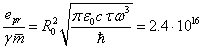 C/kg.
(40)
C/kg.
(40)
In Section 6, we have shown
how the praon’s charge and mass are calculated from the theory of similarity of
matter levels with the use of similarity coefficients. If we substitute ![]() in (40), then we would find the value of the
Lorentz factor
in (40), then we would find the value of the
Lorentz factor ![]() .
.
For the case of a
hydrogen-like atom we can see that in (40) the following proportions hold true:
![]() according to (7), as well
according to (7), as well ![]() and
and ![]() . If the
principal quantum numbers of the energy states
. If the
principal quantum numbers of the energy states ![]() and
and ![]() are large enough, and the condition
are large enough, and the condition ![]() is met, then we will have
is met, then we will have ![]() .
Consequently, the Lorentz factor
.
Consequently, the Lorentz factor ![]() increases in proportion to the nuclear charge
number
increases in proportion to the nuclear charge
number ![]() or to the square root of the photon energy:
or to the square root of the photon energy: ![]() . The
highest value
. The
highest value ![]() of the photon is expected in
the hydrogen-like atom, which has the nucleus with the largest number of
protons, and in electron transitions near the smallest orbits. In this case the
largest fields of the atom influence the praons of the emerging photon and
transfer their energy to them.
of the photon is expected in
the hydrogen-like atom, which has the nucleus with the largest number of
protons, and in electron transitions near the smallest orbits. In this case the
largest fields of the atom influence the praons of the emerging photon and
transfer their energy to them.
From transformations of the
electromagnetic field components (36) it was found that ![]() in the photon. Deriving (34) we assumed that
in the photon the balance is achieved between the electromagnetic force and the
force from the strong gravitation, and in (37) we also took into account the
equality of the electromagnetic force and the centripetal force, arising from
rotation of the praons inside the photon. The full balance of the forces should
also include the fourth force, arising from repulsion of the praons’ charges
from each other. All the four forces are approximately equal in magnitude. Let
us now consider the ratio of the energy fluxes inside the photon. For the
average values of the electromagnetic Poynting vector and accordingly of the
gravitational Heaviside vector [12], [19], after averaging over the wave period of the periodically varying
field components, we can write:
in the photon. Deriving (34) we assumed that
in the photon the balance is achieved between the electromagnetic force and the
force from the strong gravitation, and in (37) we also took into account the
equality of the electromagnetic force and the centripetal force, arising from
rotation of the praons inside the photon. The full balance of the forces should
also include the fourth force, arising from repulsion of the praons’ charges
from each other. All the four forces are approximately equal in magnitude. Let
us now consider the ratio of the energy fluxes inside the photon. For the
average values of the electromagnetic Poynting vector and accordingly of the
gravitational Heaviside vector [12], [19], after averaging over the wave period of the periodically varying
field components, we can write:
![]() ,
, ![]() ,
, ![]() ,
, ![]() ,
,
here ![]() is the vector of the gravitational torsion
field as the strong gravitational field component, which is similar in its meaning
to the magnetic field induction, and we used the conditions of the form
is the vector of the gravitational torsion
field as the strong gravitational field component, which is similar in its meaning
to the magnetic field induction, and we used the conditions of the form ![]() and
and ![]() for the amplitudes of the field components.
for the amplitudes of the field components.
Let us calculate the ratio of
the amplitude of the average value of the gravitational energy flux vector to
the amplitude of the average value of the electromagnetic energy flux vector. Again,
we will consider the model of a lobe inside the photon in the form of a
capacitor, as in derivation of (34), and will take into account the expressions
for the amplitudes of the field strengths in the form: ![]() and
and ![]() . In view of the relation
. In view of the relation ![]() and (34) we obtain:
and (34) we obtain:
 .
.
The ratio of the fluxes of
gravitational and electromagnetic energies in the photon turns out to be equal to
the ratio of the proton mass to the electron mass. This correlates with the
fact that, according to [14], for each matter level the ratio of the energy
density of the field of gravitons in the vacuum field, responsible for the
gravitational forces, to the energy density of the charged particles in the
vacuum field, responsible for the electromagnetic forces, is also equal to the
ratio of the proton mass to the electron mass.
8. The magnetic dipole moment
The non-zero component of the
magnetic field ![]() inside the photon leads to the fact that the
photon as a whole must have some magnetic dipole moment. Let us consider the
photon in the reference frame
inside the photon leads to the fact that the
photon as a whole must have some magnetic dipole moment. Let us consider the
photon in the reference frame ![]() , where the
amplitude of the wave vector and the wavelength, in view of (29), are as
follows:
, where the
amplitude of the wave vector and the wavelength, in view of (29), are as
follows:
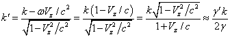 ,
, ![]() . (41)
. (41)
To estimate the magnetic field
we will represent the photon in the reference frame ![]() in the form of a solenoid with the length
in the form of a solenoid with the length ![]() that contains
that contains ![]() turns. In the reference frame
turns. In the reference frame ![]() , associated
with the photon, in each turn there is a current
, associated
with the photon, in each turn there is a current ![]() . Here
. Here ![]() is the duration of the photon emission from
the atom,
is the duration of the photon emission from
the atom, ![]() denotes the number of particles carrying the
praon’s charge
denotes the number of particles carrying the
praon’s charge ![]() in one turn, and the product
in one turn, and the product ![]() determines the total number of charges,
involved in the magnetic field creation.
determines the total number of charges,
involved in the magnetic field creation.
The mass ![]() in (38) is a certain effective mass and is
close to the praon mass
in (38) is a certain effective mass and is
close to the praon mass ![]() ; the
difference between these masses is due to the fact that the photon is not a
solid cylinder but a helical structure. Besides, the cross section of the
photon in Figure 4 has the form of lobes, and the mass density in the lobes
must be a function of the distance from the axis
; the
difference between these masses is due to the fact that the photon is not a
solid cylinder but a helical structure. Besides, the cross section of the
photon in Figure 4 has the form of lobes, and the mass density in the lobes
must be a function of the distance from the axis ![]() . In the
reference frame
. In the
reference frame ![]() the angular momentum is written as in (38),
and taking into account (35) and (38) we have:
the angular momentum is written as in (38),
and taking into account (35) and (38) we have:
![]() . (42)
. (42)
The magnetic field inside a
long solenoid depends only on the number of turns per unit length ![]() and on the flowing current
and on the flowing current ![]() :
:
![]() .
.
Substituting here ![]() ,
using (35) and (41), and expressing
,
using (35) and (41), and expressing ![]() in terms of
in terms of ![]() from (42), we find:
from (42), we find:
![]() . (43)
. (43)
If we substitute here the data
for the photon under consideration: ![]() ,
, ![]() ,
, ![]() s,
s, ![]() ,
, ![]() C, and if instead of
C, and if instead of ![]() we use the praon mass
we use the praon mass ![]() kg, we
obtain the estimate of the longitudinal magnetic field inside the photon:
kg, we
obtain the estimate of the longitudinal magnetic field inside the photon: ![]() T.
T.
The magnetic field in the
reference frame ![]() is associated with a certain effective current
is associated with a certain effective current
![]() in the turns of the solenoid, which models the photon:
in the turns of the solenoid, which models the photon:
![]() .
.
We introduce the effective
current into consideration because the charged praons in ![]() do not just revolve around the axis
do not just revolve around the axis ![]() , but also
fly along this axis at the velocity
, but also
fly along this axis at the velocity ![]() . Taking
into account the above-mentioned and the ratios
. Taking
into account the above-mentioned and the ratios ![]() and (43), on the assumption
and (43), on the assumption ![]() , we find a
dipole magnetic moment of the photon of insignificant value in the reference
frame
, we find a
dipole magnetic moment of the photon of insignificant value in the reference
frame ![]() :
:
 A·m2.
(44)
A·m2.
(44)
If the negative praons move as
is shown in Figure 4, and the photon propagates in the positive direction of
the axis ![]() ,
then the magnetic moment of the photon would be directed in the negative
direction of the axis
,
then the magnetic moment of the photon would be directed in the negative
direction of the axis ![]() and opposite to the photon velocity. If the
photon propagates oppositely to the axis
and opposite to the photon velocity. If the
photon propagates oppositely to the axis ![]() , the direction
of the magnetic moment and the velocity of the photon will coincide.
, the direction
of the magnetic moment and the velocity of the photon will coincide.
The ratio of
the magnetic moment of the photon under consideration to the Bohr magneton is
equal to ![]() .
Note that in [20], based on the astrophysical data,
there is a restriction of the magnetic dipole moment of the photon, which must
not exceed
.
Note that in [20], based on the astrophysical data,
there is a restriction of the magnetic dipole moment of the photon, which must
not exceed ![]() . In the
previous section we found that the Lorentz factor
. In the
previous section we found that the Lorentz factor ![]() increases in proportion to the nuclear charge
number
increases in proportion to the nuclear charge
number ![]() in the hydrogen-like atom or in proportion to
the square root of the photon energy:
in the hydrogen-like atom or in proportion to
the square root of the photon energy: ![]() . Then from
(44) it follows that the low-energy photons have an increased magnetic moment.
In addition, the magnetic moment of the photon must increase in transitions
with large quantum numbers
. Then from
(44) it follows that the low-energy photons have an increased magnetic moment.
In addition, the magnetic moment of the photon must increase in transitions
with large quantum numbers ![]() ,
corresponding to the electron orbits, which are distant from the nucleus.
,
corresponding to the electron orbits, which are distant from the nucleus.
In [9] we studied the
structure of various neutrinos and the ways of their formation, and it was
shown that the muon and electron neutrinos contain the fluxes of the same
particles (electron neutrinos of the praon level of matter) and differ in the
energy spectrum and in the method of ordering (helicity) of the angular momenta
of these particles as well as their fluxes in space. Due to this, electron and
muon neutrinos can partially transform into each other. Neutrinos emerge in the
weak interaction processes and differ from photons by their internal structure.
Photons are most often generated during interaction of the praons’ fluxes of
the vacuum field with the accelerated lepton matter; and neutrinos are more
typical for the processes inside the hadrons matter.
Despite the different
structures of the photon and neutrino, we assume that neutrinos of the atomic
level of matter, like photons, consist of praons and have a magnetic moment.
Therefore we will present the estimates of the dipole magnetic moment of
neutrinos: not more than ![]() ,
according to [21]; not more than
,
according to [21]; not more than ![]() , according
to [22]; not more than
, according
to [22]; not more than ![]() , according
to [23]. As we can see, the dipole
magnetic moment (44) for the photon in the hydrogen atom does not exceed the
values, which is expected for the neutrino.
, according
to [23]. As we can see, the dipole
magnetic moment (44) for the photon in the hydrogen atom does not exceed the
values, which is expected for the neutrino.
9. The photon mass
In the special theory of
relativity there is a well-known formula, connecting the relativistic energy ![]() ,
momentum
,
momentum ![]() and invariant mass
and invariant mass ![]() (the rest mass) of the particle:
(the rest mass) of the particle:
![]() . (45)
. (45)
In [24] the restriction was given for the photon’s
rest mass: ![]() eV/s2
in energy units, and in [25] it is assumed
that
eV/s2
in energy units, and in [25] it is assumed
that ![]() eV/s2.
As a rule, it is believed that the rest mass of the photon is zero,
eV/s2.
As a rule, it is believed that the rest mass of the photon is zero, ![]() , and then
the photon energy depends only on its momentum:
, and then
the photon energy depends only on its momentum: ![]() . The latter
ratio allows us to find the photon’s momentum using the energy or angular
frequency of the photon. In this case the photon must move at the speed of
light
. The latter
ratio allows us to find the photon’s momentum using the energy or angular
frequency of the photon. In this case the photon must move at the speed of
light ![]() .
.
Let us consider the case of
the photon mass in the substantial model described above. From (38) we can
determine the relativistic energy of the particles inside the photon by
multiplying the number of praons by the average rest mass of one particle ![]() , by
the Lorentz factor and by the square of the speed of light:
, by
the Lorentz factor and by the square of the speed of light:
![]() . (46)
. (46)
In (46) ![]() denotes the angular frequency of the photon,
denotes the angular frequency of the photon, ![]() is the photon energy, and the product
is the photon energy, and the product ![]() in its meaning is the averaged speed of
rotation of the electron in the atom during the photon emission. Consequently,
the relativistic energy of praons is
in its meaning is the averaged speed of
rotation of the electron in the atom during the photon emission. Consequently,
the relativistic energy of praons is ![]() times greater than the photon energy. By the
order of magnitude, the difference between the energies
times greater than the photon energy. By the
order of magnitude, the difference between the energies ![]() and
and ![]() is about tens of thousands and more.
is about tens of thousands and more.
The invariant mass of the
photon, understood as the invariant mass of the praons that make up the photon,
in view of (46) is equal to:
![]() .
(47)
.
(47)
Substituting into (46) and
(47) the data for the photon, emitted by the hydrogen atom during the
electron’s transition from the second to the first level in the Lyman series: ![]() s-1,
s-1, ![]() ,
, ![]() , we obtain
the following estimates:
, we obtain
the following estimates: ![]() J or 170
keV,
J or 170
keV, ![]() kg or
kg or ![]() eV/c2
in energy units. It turns out that the rest mass of the photon’s particles
eV/c2
in energy units. It turns out that the rest mass of the photon’s particles ![]() is not equal to zero, though it is quite low.
is not equal to zero, though it is quite low.
In (40) it was found that ![]() ,
while
,
while ![]() and
and ![]() . Therefore,
. Therefore,
![]() , that is
the total rest mass of the particles of the emitted photon increases in the
atomic transitions with large quantum numbers
, that is
the total rest mass of the particles of the emitted photon increases in the
atomic transitions with large quantum numbers ![]() and reaches the maximum for the hydrogen atom
with the nuclear charge number
and reaches the maximum for the hydrogen atom
with the nuclear charge number ![]() .
.
Instead of (45), for the
photon we can write:
![]() .
(48)
.
(48)
Since the rest energy of the
photon’s particles ![]() is very low, in (48) the relativistic energy
of the photon’s particles
is very low, in (48) the relativistic energy
of the photon’s particles ![]() is close to the product of the momentum by the
speed of light:
is close to the product of the momentum by the
speed of light: ![]() . This is
due to the fact that the Lorentz factor
. This is
due to the fact that the Lorentz factor ![]() of the particles inside the photon is very
large.
of the particles inside the photon is very
large.
From the stated above we can
see why in (48) the rest mass of the photon’s particles ![]() is not equal to zero, while in (45) the photon
mass
is not equal to zero, while in (45) the photon
mass ![]() is equated to zero. This follows from the
difference between the energies
is equated to zero. This follows from the
difference between the energies ![]() and
and ![]() – if the energy
– if the energy ![]() is associated only with the rotation energy of
the praons inside the photon and with the energy of their fields, then the
energy
is associated only with the rotation energy of
the praons inside the photon and with the energy of their fields, then the
energy ![]() also takes into account the energy of praons’
motion at the velocity
also takes into account the energy of praons’
motion at the velocity ![]() , almost
reaching the speed of light. This additional energy is not transferred to the
praons from the electrons in the photon emission from the atom, but they had
this energy at the time of interaction of the praons’ fluxes with the electron.
Not taking into account the initial energy of praons in the energy
, almost
reaching the speed of light. This additional energy is not transferred to the
praons from the electrons in the photon emission from the atom, but they had
this energy at the time of interaction of the praons’ fluxes with the electron.
Not taking into account the initial energy of praons in the energy ![]() leads to the loss of their rest mass and to zeroing of the mass
leads to the loss of their rest mass and to zeroing of the mass ![]() in (45) for the photon. In addition, the
difference arises between the momentum of praons
in (45) for the photon. In addition, the
difference arises between the momentum of praons ![]() in (48) and the generally accepted photon
momentum
in (48) and the generally accepted photon
momentum ![]() in (45).
in (45).
Despite the fact that the rest
mass of the photon particles ![]() ,
calculated by us, significantly exceeds the estimates of the photon mass in [24] and in [25], the mass
,
calculated by us, significantly exceeds the estimates of the photon mass in [24] and in [25], the mass ![]() cannot be directly found in experiments. This
is due to the fact that during interaction of the photon with the matter, the
photon’s angular momentum of the order of
cannot be directly found in experiments. This
is due to the fact that during interaction of the photon with the matter, the
photon’s angular momentum of the order of ![]() is transferred to the matter, as well as the
corresponding energy and momentum. However, the main part of the photon energy,
involved in the relativistic motion of praons, is carried away with them at the
moment of the photon decay and its scattering into separate praons.
is transferred to the matter, as well as the
corresponding energy and momentum. However, the main part of the photon energy,
involved in the relativistic motion of praons, is carried away with them at the
moment of the photon decay and its scattering into separate praons.
We assume that the velocities ![]() of the fluxes of praons in the vacuum field
are of the order of the speed of light,
of the fluxes of praons in the vacuum field
are of the order of the speed of light, ![]() . At the
same time, the photons are moving at the velocity
. At the
same time, the photons are moving at the velocity ![]() , and we
should have
, and we
should have ![]() . Some
difference between
. Some
difference between ![]() and
and ![]() is explained by the fact that the praons in
the photon do not only move along the axis
is explained by the fact that the praons in
the photon do not only move along the axis ![]() , which is
perpendicular to the plane of the electron disk at the moment of the photon
emission, but they also rotate around this axis by some spirals. Rotation of
the praons depends on the photon frequency and energy, which should influence
the velocity of the photons
, which is
perpendicular to the plane of the electron disk at the moment of the photon
emission, but they also rotate around this axis by some spirals. Rotation of
the praons depends on the photon frequency and energy, which should influence
the velocity of the photons ![]() and lead to some initial velocity dispersion
of the photons of different frequencies.
and lead to some initial velocity dispersion
of the photons of different frequencies.
10. Conclusion
In Section 2, we show that the
frequency of the photon, emitted from the atom, is equal to the rotation
frequency of the electron cloud’s center around the nucleus, averaged with
respect to the time of the photon emission during quantum transition of the
electron from a certain state to a state with lower energy.
In Section 3 we present the
expressions for the electromagnetic field strength in the wave zone away from
the charge, rotating around a certain center, which can be used to estimate the
electromagnetic energy flux. From these, it follows that most of the energy is
emitted from the charge in the rotation axis direction. In other directions the
energy flux decreases quite rapidly in magnitude and has an oscillating
character, without producing noticeable emission.
Taking as a basis the
electromagnetic fields in the near zone and the wave zone from the
hydrogen-like atom that undergoes quantum transition, we estimate the action of
these fields on the charged particles (praons) of the vacuum field. The
electron in the substantial model of the electron [9] is considered as a disk,
and the above-mentioned fields cause rotation of the praon fluxes around an
axis, which is perpendicular to the electron disk. Based on the pattern of the
field in Section 4, in Section 5 we present the corresponding photon structure.
The positively charged praons are concentrated near the photon’s axis, and the
negatively charged praons form the helical part of the photon. Based on this
structure, with the help of the idea of strong gravitation at praon level we
solve the problem of stability of the positively and negatively charged praons
inside the photon, explaining the long-term stability of the photon by the huge
value of the strong gravitational constant ![]() .
Rotation of the negative praons inside the photon leads to the fact that
photons can easily interact with electrons and other charged particles,
exchanging the energy with each other.
.
Rotation of the negative praons inside the photon leads to the fact that
photons can easily interact with electrons and other charged particles,
exchanging the energy with each other.
The photon is emitted along
the axis of the electron disk, but some part of the energy in the form of
electromagnetic emission leaves the excited atom in other directions. This
emission is in phase with the oscillations inside the photon. The latter can
explain the results of the Young’s interference experiment with low light
intensity, when interference between single photons is observed. In this case,
each photon passes through a particular slit and the coherent emission from the
atom, associated with it, passes through another slit, which as a result gives
the interference pattern.
In Sections 6-8, we estimate
the values of the fields inside the photon, the Lorentz factor for the praons
and the energy fluxes, we calculate the longitudinal magnetic field and the
magnetic dipole moment of the photon. Here we use Lorentz transformations in
order to turn to the reference frame, moving synchronously with the photon.
We finish development of the
substantial model of the photon by considering the question of the invariant
mass of the photon, which in the special theory of relativity is assumed to be
equal to zero. In contrast, in the substantial model we calculate the rest mass
of the praons that make up the photon, which obviously cannot be zero. Using
this mass and the total momentum of the praons, we determine the relativistic
energy of these praons, which tens of thousands times exceeds the energy of the
photon in the classical theory. The difference between these energies is
explained by the fact that the generally accepted photon energy does not
include the relativistic energy of the praons, moving almost at the speed of
light. As a result, in our model the photon is described by a standard
relativistic formula, which relates its energy, momentum and the nonzero rest
mass.
According to the ordinary
interpretation, the photon is considered as an elementary particle, which is a
quantum of electromagnetic emission, and its uniqueness is enhanced by the
absence of the rest mass. In quantum electrodynamics, the photon is also a
gauge boson, while the carriers of electromagnetic interaction are considered
virtual photons. However, in [14] we have shown that the electromagnetic forces
can occur under the action exerted on the charged bodies by multiple fluxes of
praons that exist in the vacuum field. In this article we consider the
processes that take place in quantum electron transitions in the atom, which
allow forming photons from the fluxes of praons. Thus, the concept of praons
allows us not only to understand the photon structure and to find its mass, but
also to give a general explanation of the main electromagnetic phenomena.
If the photon has non-zero
mass, then how could it change our understanding of the effect of light
deflection by massive bodies under the action of gravitation? According to
[15], gravitation is explained in Le Sage’s model as the result of the action
exerted on the bodies by the fluxes of gravitons in the vacuum field. As a
whole the vacuum field consists of two components, the field of gravitons and
the field of charged praons, generating gravitational and electromagnetic
forces, respectively. The photon is an object composed of praons, tightly bound
by strong gravitation and electromagnetic forces. The fluxes of praons near
massive bodies deflect from their initial direction under the action of the
graviton field. In this case the photon is not just a flux of praons, it
carries additional energy and angular momentum, acquired at the time of
emission. Moving at relativistic velocity, the photon must be influenced by the
graviton field, just like other particles having the same velocity are
influenced by this field. For example, in the covariant theory of gravitation
[26], the full angle of deflection is
given by the formula: ![]() , where
, where ![]() is the body
mass,
is the body
mass, ![]() and
and ![]() denote the velocity and the impact parameter
of the relativistic particle at infinity. If we assume for the photon
denote the velocity and the impact parameter
of the relativistic particle at infinity. If we assume for the photon ![]() , we will
arrive at the formula
, we will
arrive at the formula ![]() , which
would be valid for the photon in the general theory of relativity as well. In
this formula, there is no dependence on the mass of the relativistic particle
or on the photon mass. Therefore, emerging of the photon’s rest mass will
change the full angle of deflection
, which
would be valid for the photon in the general theory of relativity as well. In
this formula, there is no dependence on the mass of the relativistic particle
or on the photon mass. Therefore, emerging of the photon’s rest mass will
change the full angle of deflection ![]() by a very small quantity, arising from the
difference between the photon velocity and the speed of light.
by a very small quantity, arising from the
difference between the photon velocity and the speed of light.
The substantial model provides
its solution of the wave-particle duality of the photon. As an estimate of the
number of praons in the photon we used, emitted by the hydrogen atom, we will
calculate the relation: ![]() praons.
This entire set of praons is tightly bound by the electromagnetic forces and
strong gravitation at the level of praons, ensuring the integrity and long-term
stability of the photon as a particle. On the other hand, due to its origin,
the photon represents a long and rotating in space periodic structure of small
cross section. Due to this structure, the photon exhibits wave properties, in
particular by means of its field strengths, periodically varying in space and
time.
praons.
This entire set of praons is tightly bound by the electromagnetic forces and
strong gravitation at the level of praons, ensuring the integrity and long-term
stability of the photon as a particle. On the other hand, due to its origin,
the photon represents a long and rotating in space periodic structure of small
cross section. Due to this structure, the photon exhibits wave properties, in
particular by means of its field strengths, periodically varying in space and
time.
From the stated above it also
follows that due to the small difference of the photon velocity ![]() from the speed of light, the recorded photon
velocity would not the same for observers in the reference frames, moving at
different speeds. In particular, we assume the existence of the reference frame
from the speed of light, the recorded photon
velocity would not the same for observers in the reference frames, moving at
different speeds. In particular, we assume the existence of the reference frame
![]() , in which
the longitudinal velocity of the photon as a whole is equal to zero and there is
only its proper rotation.
, in which
the longitudinal velocity of the photon as a whole is equal to zero and there is
only its proper rotation.
It is convenient to assume
that the speed of light is the limiting value for the motion of photons and
particles. In transition to the lower levels of matter (to nucleons, praons,
etc.) the Lorentz factor increases in the particles that make up the photons of
the respective matter level, while their velocities must not exceed the speed
of light. Thus the theory of relativity is applied in the theory of infinite
nesting of particles. On the other hand, if the proton is accelerated by the
electromagnetic forces, actually by the directed and concentrated fluxes of
charged, relativistically moving praons, then the proton velocity cannot exceed
the velocity of these praons. If any photon and the praons, forming it, are
moving at a velocity less than the speed of light, then the proton velocity,
accelerated by such praons, will not be able to reach the speed of light. The
relativistic praons, that in the aggregate form the field of charged particle
of the vacuum field, acquired their energy in the electromagnetic fields near
the protons and other charged particles. Only the electromagnetic field is the
basic source of relativistic charged particles at all levels of matter, and
then it turns out that all these particles are moving more slowly than the
speed of light.
According to the theory of infinite nesting of matter
and calculations with the use of similarity coefficients, the invariant mass of
a positively charged praon must be ![]() kg and the radius must be
kg and the radius must be ![]() m with the proton radius equal to
m with the proton radius equal to ![]() m, according to [18]. Apparently, in
modern experiments individual particles of such low masses and sizes cannot be
detected directly. Actually, the search for preons, as the particles that make
up quarks and leptons, and for partons, as the constituent particles of
nucleons, in experiments on scattering of particles reached only the size of
m, according to [18]. Apparently, in
modern experiments individual particles of such low masses and sizes cannot be
detected directly. Actually, the search for preons, as the particles that make
up quarks and leptons, and for partons, as the constituent particles of
nucleons, in experiments on scattering of particles reached only the size of ![]() m. This is much
larger than the expected size of praons. As a result, partons were identified
as quarks and gluons, and preons as a type of new particles were not detected
and remained to be the subject of theoretical research [27].
m. This is much
larger than the expected size of praons. As a result, partons were identified
as quarks and gluons, and preons as a type of new particles were not detected
and remained to be the subject of theoretical research [27].
In our opinion, the maximum
possible photon energy ![]() , as
well as the invariant mass of its particles
, as
well as the invariant mass of its particles ![]() , depend
significantly on the way of the photon formation. If in (39) we equate the
doubled density
, depend
significantly on the way of the photon formation. If in (39) we equate the
doubled density ![]() of the electromagnetic energy inside the
photon to the energy density of the charged particles of the vacuum field
of the electromagnetic energy inside the
photon to the energy density of the charged particles of the vacuum field ![]() , and take
from [14] the value
, and take
from [14] the value ![]() J/m3,
we can estimate the maximum amplitude of the electric field strength inside the
photon:
J/m3,
we can estimate the maximum amplitude of the electric field strength inside the
photon:
 V/m.
(49)
V/m.
(49)
In (49) it is assumed that the
charged particles of the vacuum field (praons) are part of the photons at the time
of their formation, and the energy density of the photons ![]() cannot exceed the energy density
cannot exceed the energy density ![]() . The latter
follows from the fact that
. The latter
follows from the fact that ![]() is associated with rotation of the praons
inside the photon, where the rotation speed does not exceed the speed of light,
and
is associated with rotation of the praons
inside the photon, where the rotation speed does not exceed the speed of light,
and ![]() is the averaged energy density of the praons
in their motion at the velocity of the order of the speed of light. The
electric field strength (49) can be compared only with the field strength at
the surface of the proton, where
is the averaged energy density of the praons
in their motion at the velocity of the order of the speed of light. The
electric field strength (49) can be compared only with the field strength at
the surface of the proton, where ![]() V/m.
Therefore, formation of high-energy photons can be associated with the
relativistic protons and interactions with them, as is the case with the cosmic
rays.
V/m.
Therefore, formation of high-energy photons can be associated with the
relativistic protons and interactions with them, as is the case with the cosmic
rays.
In [15] we estimated the
temperature of the graviton field, which is part of the vacuum field, for the
case when gravitons are the particles similar to photons: ![]() K.
Let us assume that the field of the charged particles of the vacuum field has
the same temperature as the graviton field, and both fields are in temperature
equilibrium. Assuming in a first approximation, that the Wien's displacement
law holds true for the wavelength
K.
Let us assume that the field of the charged particles of the vacuum field has
the same temperature as the graviton field, and both fields are in temperature
equilibrium. Assuming in a first approximation, that the Wien's displacement
law holds true for the wavelength ![]() , that the
majority of photons have at the given temperature
, that the
majority of photons have at the given temperature ![]() , with
regard to the Wien's displacement constant
, with
regard to the Wien's displacement constant
![]() m·K, we find:
m·K, we find:
![]() ,
, ![]() J.
J.
In terms of energy units of
particle physics the average photon energy equals ![]() GeV
and belongs to the range of gamma-quanta. Assuming that in (37-38) the radius
GeV
and belongs to the range of gamma-quanta. Assuming that in (37-38) the radius ![]() can be replaced by the proton radius
can be replaced by the proton radius ![]() and the speed of light can be used as the
limiting speed of praons’ rotation in the photon:
and the speed of light can be used as the
limiting speed of praons’ rotation in the photon: ![]() , then for
the maximum energy of such a photon we find:
, then for
the maximum energy of such a photon we find: ![]() GeV.
GeV.
However, measurements show
that the energy of photons can be much higher and can reach 80 TeV [28].
Apparently, the photons with such energies are formed not under condition of
temperature equilibrium between the matter and electromagnetic field, but under
strongly non-equilibrium conditions. This requires interaction of a
relativistic particle with a great number of particles at the same time. The
examples are the synchrotron emission of a charged particle in the magnetic
field of a sufficiently large and magnetized object, and the inverse Compton
effect.
References
1.
R. Nisius. The photon structure from deep inelastic electron photon
scattering. Physics Report, 332,165 (2000). http://dx.doi.org/10.1016/S0370-1573(99)00115-5.
2.
T. Yarman, C. Yesilyurt and M. Arik. A Novel Photon Model – Featuring an
Internal Dynamics along with an Amplitude of the Oscillating Particle of Light.
Acta Physica Polonica A 125 (2),
638 (2014). http://dx.doi.org/10.12693/APhysPolA.125.638.
3.
Masroor H. S. Bukhari. A phenomenological model for photon mass
generation in vacuo. International Journal of Physical Sciences. 9 (4), 48 (2014). http://dx.doi.org/10.5897/IJPS2013.4025.
4.
Hongrui Li. Continuing research on the classical spiraling photon model.
Proc. SPIE 9277, (2014). http://dx.doi.org/10.1117/12.2070574.
5.
I. Bersons. Soliton Model of the Photon / Fotona Solitona Modelis.
Latvian Journal of Physics and Technical Sciences. 50 (2), 60 (2013). http://dx.doi.org/10.2478/lpts-2013-0013.
6.
P. Kamenov and B.
Slavov. A Soliton-like Model for the Photon. Bulgarian Journal of Physics. 23, 116 (1996).
7.
G. Hunter and R.L.P.
Wadlinger. Photons and Neutrinos as Electromagnetic Solitons. Physics Essays. 2, 158 (1989).
8.
Melike B. Yucel and Nuri
Unal. First quantized electron and photon model of QED and radiative processes.
Can. J. Phys. 80 (8), 803 (2002). http://dx.doi.org/10.1139/p02-027 .
9.
Sergey Fedosin, The
physical theories and infinite hierarchical nesting of matter, Volume 1, LAP LAMBERT Academic Publishing, pages:
580, ISBN-13: 978-3-659-57301-9. (2014).
10.
Landau, L.D., Lifshitz
E.M. (1975). The Classical Theory of Fields (Vol. 2, 4th ed.).
Butterworth-Heinemann.
11. Feynman
R, Leighton R, and Sands M. The Feynman Lectures on Physics. Volume 2. Mainly
electromagnetism and matter. Addison-Wesley, Reading, MA. 1966.
12.
Fedosin S. G. Fizika
i filosofiia podobiia ot preonov do metagalaktik. (Perm,
1999). ISBN 5-8131-0012-1.
13. Fedosin S.G. Cosmic Red Shift, Microwave Background, and New
Particles. Galilean
Electrodynamics, Spring 2012, Vol. 23, Special Issues No. 1, P. 3 – 13.
14. Fedosin S.G. The charged component of the vacuum field
as the source of electric force in the modernized Le Sage’s model. Journal of
Fundamental and Applied Sciences, Vol. 8, No. 3, P. 971-1020 (2016). http://dx.doi.org/10.4314/jfas.v8i3.18.
15. Fedosin S.G. The graviton field as
the source of mass and gravitational force in the modernized Le Sage’s model.
Physical Science International Journal. Vol. 8, Issue 4, P. 1-18 (2015). http://dx.doi.org/10.9734/PSIJ/2015/22197.
16. Fedosin S.G. Four-Dimensional Equation of Motion for Viscous
Compressible and Charged Fluid with Regard to the Acceleration Field, Pressure
Field and Dissipation Field.
International Journal of Thermodynamics. Vol. 18 (No. 1), pp. 13-24, 2015. http://dx.doi.org/10.5541/ijot.5000034003.
17. Fedosin
S.G. The Hamiltonian in Covariant Theory of
Gravitation. Advances in Natural
Science, 2012, Vol. 5, No. 4, P. 55 – 75. http://dx.doi.org/10.3968%2Fj.ans.1715787020120504.2023.
18. Fedosin
S.G. The radius of the proton in
the self-consistent model. Hadronic
Journal, 2012, Vol. 35, No. 4, P. 349 – 363.
19. O. Heaviside (1893). A gravitational and electromagnetic
analogy. The
Electrician 31: 81–82.
20. Brett
Altschul. Astrophysical bounds on the photon charge and magnetic moment.
Astroparticle Physics, 2008, Vol. 29, Issue 4, P. 290–298. http://dx.doi.org/10.1016/j.astropartphys.2008.02.006 .
21. MUNU
Collaboration, Z. Daraktchieva et. al. Final results on the neutrino magnetic
moment from the MUNU experiment. Phys. Lett. B615 (2005), 153–159. http://dx.doi.org/10.1016/j.physletb.2005.04.030.
22. G. G.
Raffelt. New bound on neutrino dipole moments from globular cluster stars,
Phys. Rev. Lett. 64 (1990), 2856–2858. http://dx.doi.org/10.1103/PhysRevLett.64.2856.
23. N. F.
Bell, V. Cirigliano, M. J. Ramsey-Musolf, P. Vogel, and M. B. Wise. How
magnetic is the Dirac neutrino? Phys. Rev. Lett. 95 (2005), 151802. http://dx.doi.org/10.1103/PhysRevLett.95.151802.
24. E. Williams, J. Faller and H. Hill.
New Experimental Test of Coulomb's Law: A Laboratory Upper Limit on the Photon
Rest Mass. Physical Review Letters, 26
(12), 721 (1971). http://dx.doi.org/10.1103/PhysRevLett.26.721.
25. Particle Data Group, Amsler, C. et
al. Damour et al. (2008 +2009 partial update). Review of Particle Physics:
Gauge and Higgs bosons. Physics Letters B 667:
1. http://dx.doi.org/10.1016/j.physletb.2008.07.018.
26. Sergey
Fedosin, The physical theories and infinite
hierarchical nesting of matter, Volume 2, LAP LAMBERT Academic
Publishing, pages: 420, ISBN-13: 978-3-659-71511-2. (2015).
27. V. V.
Burdyuzha. The fractal universe, preon structure of particles, and the familon
model of dark matter. Astronomy Reports, 2014, Vol. 58, Issue 6, P. 353-362. http://dx.doi.org/10.1134/S106377291406002X.
28. F. Aharonian et al. (The HEGRA Collaboration). The
Crab Nebula and Pulsar between 500 GeV and 80 TeV: Observations with the HEGRA
stereoscopic air Cherenkov telescopes. The Astrophysical Journal, 614 (2), 897–913 (2004). http://dx.doi.org/10.1086/423931.
Source: http://sergf.ru/mfen.htm