Advances in Physics Theories and
Applications, Vol. 44, P. 123 – 138 (2015). http://iiste.org/Journals/index.php/APTA/article/view/23040
Generation
of Magnetic Fields in Cosmic Objects: Electrokinetic Model
Sergey
G. Fedosin
Sviazeva Str. 22-79, Perm 614088, Russia
Tel: +7912-987-04-08 E-mail: intelli@list.ru
Received:
2015-06-11
Accepted:
2015-06-22
Published:
2015-06-30
Abstract
Based on the assumption of
separation of the charges in matter of cosmic bodies the
possibility of obtaining the magnetic moment by these bodies is proved. The
magnitude of the magnetic field appears proportional to the angular velocity of
the body’s rotation and to the radius of convective layer. The periods of
change of polarity of magnetic field of the Earth and the Sun are calculated by
means of the size the convective layer and the convection speed. The solar
activity appears the consequence of periodic transformation of the thermal
energy into the electromagnetic form of energy.
Keywords: electrokinetic model, stellar magnetic fields,
geomagnetism
1. Introduction
One of the most popular theories on the ways of
generation of the magnetic field of cosmic bodies is the theory of
hydromagnetic dynamo (HD). In 1919 the English physicist J. Larmor
first suggested this idea to explain the solar magnetic field (Larmor 1919). For the theory of HD it is essential that the
ionized fluid was moving in a special, rather complicated way under the action
of internal pressure, the buoyancy force, gravitation and magnetic forces. For
example, the existing magnetic field "frozen into the fluid
" due to the effect of induction, together with the fluid should
turn with the formation and superposition of loops of the magnetic field (Vainshtein and Zel'dovich 1972).
Then the addition of the magnetic fields of the adjacent matter units and
increase of the total magnetic field are possible. There are a number of
solutions of equations of magnetohydrodynamics for HD and geodynamo
simulations, when with the given matter fluxes increasing and maintaining of
the magnetic field takes place (Kono and Roberts 2002). But so far there is no evidence that the
actual motion of electroconductive and magnetized matter in cosmic bodies could
correspond to the motions required for the effect of HD (Tobias 2002). Recent developments include numerical models of
the solar convection zone and outer radiative
interior that capture the convective motions and rotation and begin to show
cycling dynamo behaviour, though they do not yet succeed in producing
solar-like behavior: either they need a rotation rate
that is far greater than that of the Sun, or they produce cycle periods that
are longer than the Sun’s (Thompson 2014).
We shall now point out the scales of the energy
required for the effect of HD in the Earth interior. Measurements of the
Earth's magnetic field show that its main sources are hidden in the core, and
the magnitude of the field changes slowly with the time. To characterize the
sizes of the Earth we shall use the following approximate data: the average
radius is 6371 km, the equatorial radius – 6378 km, the polar radius – 6356 km.
In 2005, at the north magnetic pole of the Earth (near the coast of the
Canadian Archipelago), the magnetic field induction
was about ![]() T according to the
World Magnetic Model of the Earth (British Geological Survey 2005). Assuming that this field is generated by
the magnetic dipole moment, using the polar radius
T according to the
World Magnetic Model of the Earth (British Geological Survey 2005). Assuming that this field is generated by
the magnetic dipole moment, using the polar radius ![]() of the Earth, we can
estimate the magnetic moment of the Earth:
of the Earth, we can
estimate the magnetic moment of the Earth: ![]() J/T, where
J/T, where ![]() is the vacuum
permeability.
is the vacuum
permeability.
The inner crystalline core of the Earth has the radius
of the order of ![]() km, and the outer
liquid core of molten iron can be presented as part of the ball between the
radius
km, and the outer
liquid core of molten iron can be presented as part of the ball between the
radius ![]() and the radius
and the radius ![]() km, with the mass of
about
km, with the mass of
about ![]() kg (Жарков 1978). In the outer
core the currents should presumably flow, maintaining the magnetic field due to
the effect of HD. The magnetic moment of the Earth can be modeled by the
product of the electric current and the area of the contour of the outer core
(the core section). Hence, the required electric current should be of the order
of
kg (Жарков 1978). In the outer
core the currents should presumably flow, maintaining the magnetic field due to
the effect of HD. The magnetic moment of the Earth can be modeled by the
product of the electric current and the area of the contour of the outer core
(the core section). Hence, the required electric current should be of the order
of ![]() A. The conductivity of
the core fluid, with the value of up to
A. The conductivity of
the core fluid, with the value of up to ![]() S/m according to (Жарков 1978), allows to
estimate the electrical resistance of the fluid, which is proportional to the
length of the circumference of the core and inversely proportional to half of
its section:
S/m according to (Жарков 1978), allows to
estimate the electrical resistance of the fluid, which is proportional to the
length of the circumference of the core and inversely proportional to half of
its section: ![]() .
.
Then the power of electrical losses due to the current
flow should reach ![]() W. As we have
mentioned in (Fedosin 2014), the total heat flow from the Earth's
surface is equal to 3.2·1013 W, the contribution into the thermal
energy of the Earth from lunar tides can be up to 3.45·1012 W, and
the average power of seismicity of the Earth is about 3·1010 W.
Thus, the thermal energy would be sufficient to start the HD mechanism.
W. As we have
mentioned in (Fedosin 2014), the total heat flow from the Earth's
surface is equal to 3.2·1013 W, the contribution into the thermal
energy of the Earth from lunar tides can be up to 3.45·1012 W, and
the average power of seismicity of the Earth is about 3·1010 W.
Thus, the thermal energy would be sufficient to start the HD mechanism.
But apparently, the theory of HD may not be the
general theory to explain the magnetic field of all cosmic bodies, since in
white dwarfs and neutron stars, convection is almost absent, while the magnetic
fields of these stars are extremely high. There is no significant motion of
matter in the solar interior, where the main energy transfer from the core to
the outside occurs due to emission, and for photons it takes several million
years. Only in the solar shell convection is so large that it leads to the
periodic removal of the magnetic field tubes to the surface, which produce
sunspots there. However, the observed changes in the polarity of the magnetic
field of the Sun (with a period of about 22 years) and the Earth (with periods
from 20,000 years up to a million years or more) contradict the theory of HD.
Indeed, the effect of HD requires initial magnetic field, which can then be
amplified and further be maintained by the motion of fluid of the same type. In
the change of the polarity the magnetic field should be systematically reduced
to zero, thereby eliminating the initial magnetic field, which is necessary for
the occurrence of HD.
In
this regard, we present further electrokinetic model of the origin of the
magnetic field in space objects, as some additional mechanism which is
independent on the hydrodynamic dynamo.
2. The electrokinetic model
According to the results in (Fedosin 2012, 2014), the
magnetic moment of the proton can be obtained from the condition that the
electric charge of the proton is almost uniformly distributed over its volume.
Then the rapid rotation of the proton with its volume electric charge is able
to generate the required magnetic moment. In addition, the highly magnetized
matter of the proton is also involved in the creation of the magnetic moment of
the proton. The analogy here is the neutron stars-magnetars, the magnetic
moment of which is made up of the magnetic moments of the neutrons, which form
the basis of the stellar matter. In order the proton and the magnetar could
obtain the corresponding electrical charges and the magnetic moments with
almost total magnetization of their matter, appropriate conditions are
necessary. In particular, the proton can occur from the neutron in beta decay,
when the negative charge is removed from the neutron due to emission of the
electron. As the model of the neutron in (Fedosin 2014) the
neutron star was considered, in which due to the process of charge separation
the core becomes positively charged and the shell obtains the negative charge.
It allowed explaining the neutrality of the neutron and its negative magnetic
moment. The neutron star can obtain a sufficiently large magnetic field already
at its formation in the collapse of the supernova core, as the star rotates
rapidly and also accumulates the magnetic flux of the original star.
Based on these data, we shall construct the
electrokinetic model of emerging of the magnetic field of the Earth. The name
of the model implies that a significant role in it is played by the
distribution of electric charges and their motion as the sources of the
magnetic field. It is known that the closer we get to the center of the Earth,
the higher is the temperature of the matter. At the Earth's surface the
temperature gradient is about 20 degrees per 1 km, in the depth the gradient
decreases. The average temperature of the Earth core is in the range of 5000 –
6000º K, and on the outer core radius ![]() the expected change in
the temperature reaches 2000º K. Thus, the temperature gradient can lead to
diffusion of free electrons to the outer shell of the outer core, where the
temperature is lowered. This effect can be caused by the pressure gradient in
the matter ionized by the high temperature, which pushes the electrons out
faster than the ions.
the expected change in
the temperature reaches 2000º K. Thus, the temperature gradient can lead to
diffusion of free electrons to the outer shell of the outer core, where the
temperature is lowered. This effect can be caused by the pressure gradient in
the matter ionized by the high temperature, which pushes the electrons out
faster than the ions.
We shall suppose that for the matter the formula for
the pressure of the ideal gas is valid: ![]() , where
, where ![]() is the concentration
of particles,
is the concentration
of particles, ![]() is the Boltzmann
constant,
is the Boltzmann
constant, ![]() is temperature.
According to (Жарков 1978), the pressure
in the center of the Earth reaches 3600 kb, and at the periphery of the outer
core it is 1350 kb, with the corresponding temperatures of 6300º K and 4300º K.
From these data and the formula for the pressure it follows that the ratio of
the concentration of the particles of matter at the border of the outer core to
the concentration in the center of the Earth can be in the range 0.55 – 0.75
(the latter figure is closer to the standard physical models of the Earth
structure). The presence of gradients of concentration, pressure and
temperature (as well as the centripetal force due to the Earth’s rotation and
chemical separation which changes the buoyancy of fluid) leads to emerging of
radial flows of matter, including the currents of ions and electrons. The thermal
velocities of electrons are much higher than the ion velocities, so the
electron diffusion can occur faster.
is temperature.
According to (Жарков 1978), the pressure
in the center of the Earth reaches 3600 kb, and at the periphery of the outer
core it is 1350 kb, with the corresponding temperatures of 6300º K and 4300º K.
From these data and the formula for the pressure it follows that the ratio of
the concentration of the particles of matter at the border of the outer core to
the concentration in the center of the Earth can be in the range 0.55 – 0.75
(the latter figure is closer to the standard physical models of the Earth
structure). The presence of gradients of concentration, pressure and
temperature (as well as the centripetal force due to the Earth’s rotation and
chemical separation which changes the buoyancy of fluid) leads to emerging of
radial flows of matter, including the currents of ions and electrons. The thermal
velocities of electrons are much higher than the ion velocities, so the
electron diffusion can occur faster.
It seems that if in the matter the separation of the
charges takes place under action of different factors, then the electric force
between the positive and the negative ions should counteract this separation,
and at some point stop it. However, in the case of complete spherical symmetry,
this occurs in a special way. We shall suppose, for definiteness, that in the
center of the sphere there is a positive charge, and a negative charge equal to
it by the value is dispersed throughout the sphere. It turns out that near the
surface of the sphere, the electrons are in equilibrium, since the action of
the internal positive charge will be compensated by the action of the total
negative charge. In moving inside of the sphere the relative equilibrium of the
electrons can be maintained up to the radius at which the electric and
gravitational forces of attraction to the center are compensated by the force of
repulsion of the electrons from each other and by the gradients of temperature
and pressure. We can notice that a similar structure of separated charges is
realized in the electron-ion model of ball lightning, in which the lightning
consists almost entirely of the positively charged ionized hot air with a thin
shell of electrons. The stability of the electrons is provided by their rapid
rotation and the electrical forces, and the electron shell shields the
lightning from the surrounding atmosphere (Fedosin 2001, 2002).
We shall assume in our simple idealized model, that
under the influence of several factors the separation of charges took place in
the Earth's core. This could occur even at the time of formation of the Earth,
when it had high temperature and was nearly all melted. We shall use the linear
formula for the distribution of the total charge density: ![]() , where
, where ![]() is the charge density
in the center,
is the charge density
in the center, ![]() is some coefficient,
is some coefficient, ![]() is the current radius
from the center to the arbitrary point in the core. The coefficient
is the current radius
from the center to the arbitrary point in the core. The coefficient ![]() can be determined from
the condition of the electroneutrality of the core as a whole. To do this, we
must integrate the charge density over the entire volume of the core and equate
the result to zero. After finding
can be determined from
the condition of the electroneutrality of the core as a whole. To do this, we
must integrate the charge density over the entire volume of the core and equate
the result to zero. After finding ![]() through
through ![]() and the radius of the
outer core
and the radius of the
outer core ![]() , we obtain the following formula for the charge density:
, we obtain the following formula for the charge density:
 . (1)
. (1)
At low ![]() the charge density
the charge density ![]() is positive, with
is positive, with ![]() the final charge
density becomes negative. The charge, distributed in the core according to the
relation (1) is fixed relative to the Earth and rotates with it at the angular
velocity
the final charge
density becomes negative. The charge, distributed in the core according to the
relation (1) is fixed relative to the Earth and rotates with it at the angular
velocity ![]() rad/s.
This creates the magnetic field of the Earth with the magnetic moment
rad/s.
This creates the magnetic field of the Earth with the magnetic moment ![]() . In (Fedosin 2014) we integrated the charge density
distribution of the form (1) in order to find the magnetic moment. Similarly,
for the magnetic moment of the Earth we find:
. In (Fedosin 2014) we integrated the charge density
distribution of the form (1) in order to find the magnetic moment. Similarly,
for the magnetic moment of the Earth we find:
![]() , (2)
, (2)
where ![]() is the volume of the outer core of the Earth,
is the volume of the outer core of the Earth,
and the minus sign in (2) shows that the total magnetic
moment of the Earth is directed opposite to the angular velocity of its
rotation ![]() , if the main contribution to the magnetic moment is made by
the electrons at the core periphery.
, if the main contribution to the magnetic moment is made by
the electrons at the core periphery.
From (2) by the known values ![]() J/T,
J/T,
![]() and
and ![]() it is
possible to estimate the charge density in the center of the Earth:
it is
possible to estimate the charge density in the center of the Earth: ![]() C/m3.
The charge density distribution (1) allows us to find the magnetic field in the
center of the Earth. For each elementary circular current, which arises due to
rotation of the charge
C/m3.
The charge density distribution (1) allows us to find the magnetic field in the
center of the Earth. For each elementary circular current, which arises due to
rotation of the charge ![]() at the angular velocity
at the angular velocity ![]() , in spherical coordinates we can write down:
, in spherical coordinates we can write down:
 .
.
The elementary circular currents are differently
shifted along the axis ![]() relative to the
center of the sphere with the radius
relative to the
center of the sphere with the radius ![]() of the outer
core. Their contribution to the total magnetic field in the center of the sphere
can be taken into account with the help of the angle
of the outer
core. Their contribution to the total magnetic field in the center of the sphere
can be taken into account with the help of the angle ![]() , under which each elementary circular current from
the center of the sphere relative to the axis
, under which each elementary circular current from
the center of the sphere relative to the axis ![]() is seen:
is seen:
![]() .
.
This formula is obtained from the standard expression
for the magnetic field on the axis of the elementary circular current inside
the sphere ![]() , where
, where ![]() is the radius
of the circular current,
is the radius
of the circular current, ![]() is the distance
from the center of the sphere to the center of the elementary circular current,
is the distance
from the center of the sphere to the center of the elementary circular current,
![]() , the angle
, the angle ![]() is the angular
coordinate of the spherical coordinates.
is the angular
coordinate of the spherical coordinates.
Substituting the current ![]() into the expression
for
into the expression
for ![]() and expressing
and expressing ![]() in it with the help of
(1) and the values
in it with the help of
(1) and the values ![]() from (2), after integration over the volume of the core we obtain the
magnetic field induction at the center of the Earth:
from (2), after integration over the volume of the core we obtain the
magnetic field induction at the center of the Earth:
 T, (3)
where ![]() from (2) was also
used.
from (2) was also
used.
For comparison, we shall give the magnitude of the
magnetic field induction at the equator outside the outer core, calculated by
the standard dipole formula through the magnetic moment of the Earth ![]() for the case if the
magnetic moment was at the center of the Earth:
for the case if the
magnetic moment was at the center of the Earth:
![]() T, (4)
T, (4)
here ![]() is considered
negative.
is considered
negative.
The value of the field (4) is not entirely accurate,
since the magnetic moment is actually dispersed throughout the core in a nonuniform way. Therefore, as a first approximation, we
shall assume that the magnetic field at the equator of the core is twice larger
than (4), and is equal to ![]() .
.
We can assume that the magnetic fields at the center
of the core and near the surface have opposite directions (this is the
consequence of the change in the sign of the charge density (1) when moving
along the radius from the center to the surface of the core). Then in the
motion in the equatorial plane along the radius from the center to the edge of
the outer core the magnetic field induction will change from ![]() to
to ![]() . This can be reflected by the following linear formula:
. This can be reflected by the following linear formula:
 . (5)
. (5)
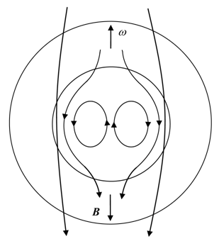
According to (5), the magnetic field changes its sign
inside the core. In accordance with these considerations Figure 1 shows a
simplified picture of the magnetic field in the Earth’s core. We shall remind
that this structure of the field is the consequence of rotation of the electric
charge distributed along the radius of the core.
We shall now estimate the average velocity of matter
motion ![]() in the Earth's
core. We shall suppose that under the influence of the temperature gradient,
the pressure force (the buoyancy force), the gravitational and centripetal
forces, the matter moves approximately along the radius. The first three forces
can be considered symmetrical relative to the center of the core, whereas the
centripetal force is symmetrical relative to the axis of rotation of the Earth.
We can therefore expect an increased speed of matter motion in the equatorial
plane of the core.
in the Earth's
core. We shall suppose that under the influence of the temperature gradient,
the pressure force (the buoyancy force), the gravitational and centripetal
forces, the matter moves approximately along the radius. The first three forces
can be considered symmetrical relative to the center of the core, whereas the
centripetal force is symmetrical relative to the axis of rotation of the Earth.
We can therefore expect an increased speed of matter motion in the equatorial
plane of the core.
During the motion of the conducting fluid in the
magnetic field, currents are induced in this fluid due to the Lorentz force. If
the magnetic field is directed along the axis ![]() , and the fluid is moving perpendicular to the axis
, and the fluid is moving perpendicular to the axis ![]() , the current density would obtain rotation around the
axis
, the current density would obtain rotation around the
axis ![]() :
:
![]() . (6)
. (6)


In our simplified approach, we shall assume the
velocity of the fluid to be constant, and as the magnetic field induction we
shall take the mean value ![]() . The maximum induced current can be estimated as the
product of the current density and the half-section of the core:
. The maximum induced current can be estimated as the
product of the current density and the half-section of the core: ![]() , where the coefficient
, where the coefficient ![]() takes into
account that the hot fluid is not only removed from the axis
takes into
account that the hot fluid is not only removed from the axis ![]() , but returns after cooling, reducing the induced
current. This current generates in the core the magnetic moment with the value:
, but returns after cooling, reducing the induced
current. This current generates in the core the magnetic moment with the value:
![]() .
(7)
.
(7)
It is obvious that the magnetic moment ![]() must be less than the
magnetic moment of the Earth:
must be less than the
magnetic moment of the Earth: ![]() , where
, where ![]() . Substituting here the absolute value
. Substituting here the absolute value ![]() from (3) in the
assumption that
from (3) in the
assumption that ![]() we find:
we find:
![]() . (8)
. (8)
From (7) and (8) for the velocity of the fluid we
obtain:
![]() m/s. (9)
m/s. (9)
The velocity of the fluid (9) is small enough. Using
it we can estimate the Reynolds number ![]() , the magnetic Reynolds number
, the magnetic Reynolds number ![]() , the magnetic Prandtl
number
, the magnetic Prandtl
number ![]() , here
, here ![]() Pa·s is the
dynamic viscosity (internal friction) in the core, according to (Жарков 1978),
Pa·s is the
dynamic viscosity (internal friction) in the core, according to (Жарков 1978), ![]() S/m is the
conductivity of the core fluid,
S/m is the
conductivity of the core fluid, ![]() kg/m3 is the average fluid density in the core.
Based on (15) further it will be shown that
kg/m3 is the average fluid density in the core.
Based on (15) further it will be shown that ![]() in (9).
Substituting the values of all quantities, we find
in (9).
Substituting the values of all quantities, we find ![]() ,
, ![]() ,
, ![]() . The Reynolds number is inversely proportional to the
adhesive force of the particles of gas or liquid, which affects the free motion
of the body or separate elements of the fluid. The magnetic Reynolds number is
directly proportional to the force of magnetic friction in the fluid that
prevents from the slippage of the magnetic lines through the fluid. The
magnetic Prandtl number is an additional
characteristic that takes into account the contributions of the magnetic and
ordinary friction and increases with increasing of viscosity and conductivity
of the fluid.
. The Reynolds number is inversely proportional to the
adhesive force of the particles of gas or liquid, which affects the free motion
of the body or separate elements of the fluid. The magnetic Reynolds number is
directly proportional to the force of magnetic friction in the fluid that
prevents from the slippage of the magnetic lines through the fluid. The
magnetic Prandtl number is an additional
characteristic that takes into account the contributions of the magnetic and
ordinary friction and increases with increasing of viscosity and conductivity
of the fluid.
We can compare the obtained numbers with the
corresponding numbers, with which the hydromagnetic dynamo (HD) can occur. For
example, in the Ponomarenko dynamo (Ponomarenko 1973) it is required that ![]() . In (Schekochihin et al
2007) it is proved that the diffusion dynamo is possible when
. In (Schekochihin et al
2007) it is proved that the diffusion dynamo is possible when ![]() and
and ![]() , and also when
, and also when ![]() and
and ![]() ,
, ![]() . If the formula (8) and our calculations of the
numbers are valid, it turns out that the conditions for the occurrence of HD in
the Earth's core are not favorable.
. If the formula (8) and our calculations of the
numbers are valid, it turns out that the conditions for the occurrence of HD in
the Earth's core are not favorable.
We shall now consider the issue of the relationship
between the magnetic force and the Coriolis force
acting on the unit of the conductive core fluid. From the value ![]() it follows that
the adhesion of the magnetic field lines to the fluid is small in the core
scale. The obtained above estimate of the value of the magnetic field in the
core is almost one order of magnitude greater than the value of the magnetic
field on the Earth's surface and in general has little effect on the motion of
the fluid. The density of the magnetic force can be written as follows:
it follows that
the adhesion of the magnetic field lines to the fluid is small in the core
scale. The obtained above estimate of the value of the magnetic field in the
core is almost one order of magnitude greater than the value of the magnetic
field on the Earth's surface and in general has little effect on the motion of
the fluid. The density of the magnetic force can be written as follows:
![]() , (10)
, (10)
where ![]() is the current
density, transferred by the fluid unit in the core, mainly in the radial
direction,
is the current
density, transferred by the fluid unit in the core, mainly in the radial
direction, ![]() is the charge density
(1).
is the charge density
(1).
For the density of the Coriolis
force, we have:
![]() .
(11)
.
(11)
The forces (10) and (11) have opposite directions and
both depend in the same way on the velocity ![]() of the fluid motion,
and the magnetic field and the angular velocity are approximately parallel. The
inertial force (11) is substantially greater than the magnetic force (10) since
the core fluid is not an ideal conductor. We shall suppose now that for all the
planets, in which the magnetic field is generated in the core, there is the
same dependence between the forces (10) and (11). Namely, we shall assume that
for the magnitudes of the densities of forces, the relation
of the fluid motion,
and the magnetic field and the angular velocity are approximately parallel. The
inertial force (11) is substantially greater than the magnetic force (10) since
the core fluid is not an ideal conductor. We shall suppose now that for all the
planets, in which the magnetic field is generated in the core, there is the
same dependence between the forces (10) and (11). Namely, we shall assume that
for the magnitudes of the densities of forces, the relation ![]() is satisfied, where
is satisfied, where ![]() . From (10) and (11) we obtain:
. From (10) and (11) we obtain:
![]() . (12)
. (12)
The fluid density ![]() in the right side of
(12) within the core does not change so significantly as the values
in the right side of
(12) within the core does not change so significantly as the values ![]() and
and ![]() in the left
side. We shall substitute instead of
in the left
side. We shall substitute instead of ![]() and
and ![]() some average
values, which make the greatest contribution. We shall assume
some average
values, which make the greatest contribution. We shall assume ![]() as the absolute
value of the double charge density from (1) with
as the absolute
value of the double charge density from (1) with ![]() . Instead of
. Instead of ![]() , we shall use
, we shall use ![]() which is equal to half
of the magnitude of the magnetic field induction at the center of the core from
(3). The equation (12) after excluding the value
which is equal to half
of the magnitude of the magnetic field induction at the center of the core from
(3). The equation (12) after excluding the value ![]() with the help of (2)
takes the following form:
with the help of (2)
takes the following form:
![]() ,
,
 .
(13)
.
(13)
If the coefficient ![]() is approximately equal
for all planets, then (13) gives the formula for determining the magnetic
moments of the planets through their known angular velocities of rotation
is approximately equal
for all planets, then (13) gives the formula for determining the magnetic
moments of the planets through their known angular velocities of rotation ![]() , the radii of the cores
, the radii of the cores ![]() and the densities of
the fluid
and the densities of
the fluid ![]() in these cores. The
dependence of the form (13) was constructed in (Fedosin
1999) and it was noted that it approximates the magnetic moments of the
planets as well as the dependence of the magnetic moments from the spins of the
cores of the planets. Even the magnetic moment of the Sun satisfies the formula
(13). We shall note that the dependence of the magnetic moment of the planet in
the form
in these cores. The
dependence of the form (13) was constructed in (Fedosin
1999) and it was noted that it approximates the magnetic moments of the
planets as well as the dependence of the magnetic moments from the spins of the
cores of the planets. Even the magnetic moment of the Sun satisfies the formula
(13). We shall note that the dependence of the magnetic moment of the planet in
the form ![]() was also found in (Busse 1976).
was also found in (Busse 1976).
We shall estimate the magnitude of the maximum
magnetic field induction at the center of the planet, substituting ![]() from (13) into (3):
from (13) into (3):
![]() . (14)
. (14)
From (14) it follows that the magnetic field in the
core is determined by the angular velocity of rotation, the radius of the core
and the fluid density. The expression (14) can be transformed, taking into
account the relation for the magnetic energy density in the center of the core ![]() and the
relation for the kinetic energy density at the equator of the core
and the
relation for the kinetic energy density at the equator of the core ![]() . This gives the following equation:
. This gives the following equation:
![]() . Therefore, approximately equal coefficient
. Therefore, approximately equal coefficient ![]() for all the planets
follows from the fact that the density of the magnetic energy contained in the
cores of the planets is proportional to the rotational kinetic energy of the
cores. In our opinion this indicates that the magnetic field is generated
rather by the rotation of the charge, which has some gradient of distribution
in the core due to the difference of temperatures and pressures than due to the
mechanism of HD. The estimate of
for all the planets
follows from the fact that the density of the magnetic energy contained in the
cores of the planets is proportional to the rotational kinetic energy of the
cores. In our opinion this indicates that the magnetic field is generated
rather by the rotation of the charge, which has some gradient of distribution
in the core due to the difference of temperatures and pressures than due to the
mechanism of HD. The estimate of ![]() can be obtained from
(13). Substituting the data for the Earth, we find
can be obtained from
(13). Substituting the data for the Earth, we find ![]() .
.
3. The Earth's magnetic field reversals
The magnetic field induction of our planet
is not constant; it fluctuates with the difference of minimum and maximum
amplitudes almost by a factor of 2, with the period of about 7500 years (the
fundamental frequency in the spectrum). There are also variations with
characteristic periods from 550 to 1800 years (Жарков
1978), explained by magnetohydrodynamic waves in the Earth's core. In
particular, the drift of isoclines of the nondipole part
of the magnetic field to the west occurs at the speed of 0.2º per year, making
a complete rotation every 1800 years. At the equator of the outer core it would
correspond to the velocity of the fluid motion ![]() m/s.
m/s.
In the spectrum of the geomagnetic field there are
fluctuations with a period of 60 years, coinciding in time with variations in
the rotational speed of the Earth. If we assume that the fluid in 60 years
should pass a circle with the radius equal to the radius ![]() of the inner core,
then we obtain the velocity
of the inner core,
then we obtain the velocity ![]() m/s. This velocity is
too high for the flow of fluid. But
m/s. This velocity is
too high for the flow of fluid. But ![]() coincides with the
velocity of the Alfven magnetohydrodynamic wave which
is equal to
coincides with the
velocity of the Alfven magnetohydrodynamic wave which
is equal to ![]() . If we substitute here instead of
. If we substitute here instead of ![]() the magnetic field
induction from (5) for
the magnetic field
induction from (5) for ![]() , that is magnitude of about
, that is magnitude of about ![]() , then taking into account (3) we find
, then taking into account (3) we find ![]() m/s. Thus, the
transverse magnetohydrodynamic waves near the inner
core can influence its rotation, the change of the Earth's rotational speed and
the total magnetic field, which is proportional to the angular velocity of
rotation according to (13).
m/s. Thus, the
transverse magnetohydrodynamic waves near the inner
core can influence its rotation, the change of the Earth's rotational speed and
the total magnetic field, which is proportional to the angular velocity of
rotation according to (13).
One of the reasons for the occurrence of magnetohydrodynamic waves in the Earth's core can be the
phenomena similar to the solar and lunar tides observed on the water in the
oceans and the seas. The tidal energy at their beating at large inhomogeneities of fluid can increase the energy of the
waves. If the magnetohydrodynamic waves propagate
near the surface of the outer core, then at low magnetic fields the velocities
of the waves become less. Perhaps this leads to the drift of the isoclines with
periods of about 1000 years or more, with the corresponding wave velocities,
equivalent to the fluid velocities which close to the value ![]() . The discrepancy between the directions of motion of magnetohydrodynamic waves near the inner core and at the
periphery of the outer core with each other and the direction of rotation of
the Earth, the existence of possible inhomogeneities
in the core, the fluctuations of the position of the inner core relative to the
center of the Earth and other similar factors lead to the shift of convective
flows and can cause the observed deflection of the magnetic dipole axis from
the Earth's rotation axis by about 11º, and the shift of the dipole center at
some distance from the center of the Earth. The magnetic pole is turning near
the north geographic pole: in 1580 in London the compass needle deviated from
the geographic pole to the east almost by 11º, and in 1960 – by 10º but in the
west. The opposite magnetic poles of the Earth can also be not at the same
dipole axis, but have a certain shift relative to it.
. The discrepancy between the directions of motion of magnetohydrodynamic waves near the inner core and at the
periphery of the outer core with each other and the direction of rotation of
the Earth, the existence of possible inhomogeneities
in the core, the fluctuations of the position of the inner core relative to the
center of the Earth and other similar factors lead to the shift of convective
flows and can cause the observed deflection of the magnetic dipole axis from
the Earth's rotation axis by about 11º, and the shift of the dipole center at
some distance from the center of the Earth. The magnetic pole is turning near
the north geographic pole: in 1580 in London the compass needle deviated from
the geographic pole to the east almost by 11º, and in 1960 – by 10º but in the
west. The opposite magnetic poles of the Earth can also be not at the same
dipole axis, but have a certain shift relative to it.
We shall now consider the possible causes of slow
oscillations of the magnetic field. Using the relation (9) and dividing the
radius of the outer core by the velocity of the fluid, we can find the
characteristic period of circulation of the fluid in the core:
![]() years. (15)
years. (15)
This value is close to the duration of the magnetic
field of the one polarity observed in recent historic time (about ![]() years). Consequently,
in (15) and (9)
years). Consequently,
in (15) and (9) ![]() . In the past, longer periods of one polarity often occurred,
up to a million years or more. Thus, not each circulation of the core fluid
leads to the change in the sign of the magnetic field, but rather in case of
one polarity the observed variations of the amplitude of the field take place
with the average period of about 7500 years.
. In the past, longer periods of one polarity often occurred,
up to a million years or more. Thus, not each circulation of the core fluid
leads to the change in the sign of the magnetic field, but rather in case of
one polarity the observed variations of the amplitude of the field take place
with the average period of about 7500 years.
From the perspective of electrokinetic model, the
initial charge separation (the positive charge in the center, the negative
charge at the periphery of the core) is periodically violated due to the fluid
convection. This occurs as follows. We shall suppose that the charge is
distributed in the core according to the law (1). A certain configuration of
the electric field corresponds to this charge distribution.
By solving the Poisson
equations ![]()
by the known dependence (1) of the charge density ![]() on the current
radius we can find distribution of the potential and the electric field
strength inside the Earth core:
on the current
radius we can find distribution of the potential and the electric field
strength inside the Earth core:
![]() ,
, ![]() , (16)
, (16)
provided that at the radius
![]() of outer core the electric
potential is zero, and
of outer core the electric
potential is zero, and ![]() C/m3 is the charge density in the center of the Earth.
C/m3 is the charge density in the center of the Earth.
With small radii, and also with ![]() , the electric field (16) tends to zero. The maximum
electric field is reached at
, the electric field (16) tends to zero. The maximum
electric field is reached at ![]() , that is in the middle of the outer core:
, that is in the middle of the outer core: ![]() V/m. Such a large
electric field, even with its partial neutralization can cause constant
ionization of the fluid. For comparison, in the hydrogen atom at the Bohr
radius the electric field of the nucleus is equal to
V/m. Such a large
electric field, even with its partial neutralization can cause constant
ionization of the fluid. For comparison, in the hydrogen atom at the Bohr
radius the electric field of the nucleus is equal to ![]() V/m.
V/m.
Therefore, when the maximum initial charge separation
in the Earth's core is achieved, due to ionization in the center of the core,
part of the fluid becomes positively charged and begins to move toward the
periphery of the core, mainly due to convection. At the same time the
negatively charged part of the fluid has the ability to be transferred to the
center of the core, wherein the paths of movement of the positively and negatively charged parts of the fluid do not coincide. During the time, close to the time (15),
the charge distribution in the core according to the law (1) is violated, there is partial or complete compensation of the
electric charge. To change the polarity of the magnetic field it is necessary
that such excess compensation of the electric charge would occur, with which
the new charge, which came with the fluid, took the position close to the periphery
of the core. Then the contribution of this charge in the magnetic moment would
be decisive for the sign of the magnetic field on the surface of the Earth. As
it was mentioned above, not for each time period (15) the change of the
polarity of the magnetic field takes place, it can take seven or more such
periods.
It is also possible to explain approximately in the
same way the periods of variations of the amplitude of the magnetic field with
a period of 7,500 years. In this case, if we use (15), the fluid passes a
characteristic way, which is equal ![]() , that is 20 times less than the radius of the outer core.
The hot charged fluid, circulating near the periphery of the core, comes up,
and after cooling goes back to the depth of the core, periodically changing the
total charge and the value of the magnetic field almost two times. The charge
of this fluid is not enough to change the sign of the charge of the fluid at
the periphery of the core and to change the polarity of the magnetic field
since it is taken from a limited volume. Only large-scale radial motion of the
charged fluid leads to the polarity reversal of the magnetic field of the
Earth.
, that is 20 times less than the radius of the outer core.
The hot charged fluid, circulating near the periphery of the core, comes up,
and after cooling goes back to the depth of the core, periodically changing the
total charge and the value of the magnetic field almost two times. The charge
of this fluid is not enough to change the sign of the charge of the fluid at
the periphery of the core and to change the polarity of the magnetic field
since it is taken from a limited volume. Only large-scale radial motion of the
charged fluid leads to the polarity reversal of the magnetic field of the
Earth.
We can estimate the maximum
energy of the electric field in the Earth's core, integrating over the volume
and taking into account (16) we have:
![]() J.
J.
The thermal energy and
pressure energy of the Earth's core are close to the calculated energy of the
electric field. Thus, in the core of the Earth is in principle possible charge
separation and thus the generation of the magnetic field due to the rotation of
these charges, in combination with hydromagnetic dynamo.
4. The magnetic field of the
Sun and other stars
Modern technique of measurement of the magnetic fields
allows to discover in stars relatively small details of the field and to make
medium-and large-scale magnetic topology maps. This makes it possible to
separate the poloidal (meridional) field from the toroidal field which is directed along the parallels. The
study of the magnetic configurations of young low-mass fully convective stars
in (Donati at al 2008) showed that the faster the star is rotating, the more
visible in it is the total dipole component of field on the background of
magnetic spots on the surface. For example, the dwarf V374 Peg of the spectral class M4.5 (with the
rotation period of about 12 hours, almost 60 times less than the period of
proper rotation of the Sun), has a very strong axisymmetric
magnetic field near the poles. Young newly formed stars such as T Tauri demonstrate at the pole the magnetic induction of
about tenths of Tesla, so that such axisymmetric
fields effectively regulate the flows of accretion matter from the massive
discs near these stars, as well as the jets near the poles. This picture
contradicts most theories of HD, which predict for fully convective stars the
predominance of the toroidal field component over the
poloidal. At the same time the proportionality of the magnetic field to the
angular velocity of rotation in general corresponds to our expression (14). In
solar-type stars the change of the polarity of the magnetic field, the spotted
magnetic field structure, as well as stable states with low magnetic activity
(such as the Maunder minimum for the Sun) are often observed. Many researchers
note that the magnetic field distribution is very similar in the magnetic A and
B-stars, white dwarfs and neutron stars, which suggests a common mechanism of
its formation in the stars at the stage of the main sequence, or even earlier (Reisenegger 2009).
We shall apply the electrokinetic model for
substantiation of emerging and maintaining of the solar magnetic field. With
some variations approximately 9 times per every 100 years, the field polarity
of the Sun at the poles is reversed, at the same time the 11-year cycles of
solar activity take place. Thus, every 22 years the polarity of the field is
the same, which is the full period of change in the magnetic field. The
magnetic dipole of the Sun at the maximum is estimated by the value ![]() J/T, according
to (Аллен 1977). With the average radius of the Sun
J/T, according
to (Аллен 1977). With the average radius of the Sun ![]() m we find for
this case the field induction at the pole:
m we find for
this case the field induction at the pole: ![]() T.
T.
The modern model of the Sun includes the following
main zones: 1) the core with the radius of about ![]() m (
m (![]() ), where thermonuclear reactions take place. 2) the area of radiation energy transfer with the radius from
), where thermonuclear reactions take place. 2) the area of radiation energy transfer with the radius from ![]() up to
up to ![]() m (
m (![]() ), which consists of ionized fluid. 3) the convective zone with the radius from
), which consists of ionized fluid. 3) the convective zone with the radius from ![]() and up to the
visible solar surface, i.e. up to the photosphere with a typical zone width of
about
and up to the
visible solar surface, i.e. up to the photosphere with a typical zone width of
about ![]() m. The fluid in this zone consists mainly of atoms
absorbing emission, therefore convection here is the predominant way of heat
transfer to the surface.
m. The fluid in this zone consists mainly of atoms
absorbing emission, therefore convection here is the predominant way of heat
transfer to the surface.
The feature of the Sun is the differential, not
solid-state rotation of its surface – at the equator the rotation period is
25.05 days, and at the poles the rotation period increases up to 34.3 days. For
further calculations we shall use the period of 25.38 days at the latitude of
16º, where the maximum frequency of appearance of sunspots is observed. This
gives the angular velocity of rotation ![]() rad/s
as a certain characteristic of the average solar rotation.
rad/s
as a certain characteristic of the average solar rotation.
We shall now estimate the average magnetic field
inside the Sun, based on the fact that the charge separation takes place
throughout the radial distance according to the linear approximation (1). From
(2) we find the charge density in the center in the form ![]() C/m3. Similarly, from (3) for the
magnetic field in the center of the Sun, we have:
C/m3. Similarly, from (3) for the
magnetic field in the center of the Sun, we have:
![]() T. (17)
T. (17)
Really, if there was the constant poloidal field it
cannot be stronger than a few gauss at the top of the radiative
zone, otherwise it would penetrate in the convective
zone and cause a polarity asymmetry between the two halves of the magnetic
cycle (Boruta 1996, Friedland
and Gruzinov 2004).
It turns out that the average poloidal magnetic fields inside the Sun are as
small, as in the Earth's core. The total magnetic fluxes on the solar surface
in the small-scale details are also approximately equal to the total magnetic
fluxes in the large-scale structures, giving the effective average field with
the induction ![]() T. The peak of
the field induction, discovered in separate fibers in the dark spots on the
solar surface, can be almost a thousand times greater than the magnitude of the
field (17). However, the magnetic field averaged over the entire area of a
typical sunspot, is of the order of
T. The peak of
the field induction, discovered in separate fibers in the dark spots on the
solar surface, can be almost a thousand times greater than the magnitude of the
field (17). However, the magnetic field averaged over the entire area of a
typical sunspot, is of the order of ![]() T and
significantly less than the peak values.
T and
significantly less than the peak values.
From observations of sunspots it follows that they
move faster than the surrounding plasma on the solar surface. In addition, the
newly emerging spots have an increased speed relative to the old spots. This
can be explained by the fact that in the depths the plasma rotates faster than
on the surface. The spots are connected with the deep layers by the magnetic
field, and therefore move faster, and the young spots on the average are deeper
than of the old spots. There is the profile of rotation frequency of the fluid
in the solar interior (Thompson, Christensen-Dalsgaard,
Miesch and Toomre 2003),
from which it follows that the rotation frequency at the bottom of the
convective zone is about 450 nHz.
In the fluid interaction during the convection between the different layers the exchange of the
angular momentum must take place. In equilibrium, the specific angular momentum
(the angular momentum of unit mass) will tend to a constant: ![]() . This shows that the angular velocity of rotation
. This shows that the angular velocity of rotation ![]() must be inversely
proportional to the square of the radius
must be inversely
proportional to the square of the radius ![]() and the square of the
sine of the polar angle
and the square of the
sine of the polar angle ![]() associated with the
latitude
associated with the
latitude ![]() by the expression
by the expression ![]() . But according to the profile of rotation frequency of the
fluid in the solar interior, at the equator with the latitude 0º the fluid
rotates faster when approaching the surface of the Sun, while at the surface
the rotation frequency again reduces.
. But according to the profile of rotation frequency of the
fluid in the solar interior, at the equator with the latitude 0º the fluid
rotates faster when approaching the surface of the Sun, while at the surface
the rotation frequency again reduces.
Why does the acceleration of rotation in the
convective zone take place? One of the explanations is the action of magnetic
field. From a simple linear dependence for the magnetic field of the form (5)
it follows that somewhere near the radius ![]() the magnetic
field should be minimal and should change the sign. In the convective zone the
magnetic field increases and has more significant impact on the fluid. The
total magnetic field of the Sun rotates at some average speed, specified by all
the matter in general. In its turn, the fluid tends to rotate at the same
average speed, due to the effect of partial freezing of the magnetic field
lines in the fluid. The action of the field will be more revealed where the
magnitude of the field is greater, the connection of the field with the fluid
is more and the friction of fluid layers is less. Apparently, these conditions
are best met in the equatorial area of the convective zone, which make the
largest contribution into the magnetic field and at the same time rotate
faster. According to (Rüdiger and Hollerbach
2004), a small magnetic field with induction of the order of
the magnetic
field should be minimal and should change the sign. In the convective zone the
magnetic field increases and has more significant impact on the fluid. The
total magnetic field of the Sun rotates at some average speed, specified by all
the matter in general. In its turn, the fluid tends to rotate at the same
average speed, due to the effect of partial freezing of the magnetic field
lines in the fluid. The action of the field will be more revealed where the
magnitude of the field is greater, the connection of the field with the fluid
is more and the friction of fluid layers is less. Apparently, these conditions
are best met in the equatorial area of the convective zone, which make the
largest contribution into the magnetic field and at the same time rotate
faster. According to (Rüdiger and Hollerbach
2004), a small magnetic field with induction of the order of ![]() T would be
sufficient to maintain the observed almost solid-state rotation of the zone of
radiation transfer.
T would be
sufficient to maintain the observed almost solid-state rotation of the zone of
radiation transfer.
Various estimates show that the velocities of the
fluid units in the solar convective zone are much higher than the velocities in
the Earth’s core. According to (Прохоров, Абашидзе 1986), the convection velocity at the bottom of
the convective zone is of about 1 m/s, and on the surface of the photosphere of
the Sun the velocity can reach 3 km/s. Quite a large sunspot with the size of
tens of thousands km can appear on the surface of the Sun in two or three days.
If the width of the spot is approximately equal to the path passed by the
fluid, then the average velocity of the fluid must be of the order of 100 m/s.
We can estimate the characteristic numbers describing
the motion of the fluid in the magnetic field. The quantity ![]() called the coefficient
of the magnetic diffusion at the bottom of the convective zone is not known
exactly, and presumably has the value from
called the coefficient
of the magnetic diffusion at the bottom of the convective zone is not known
exactly, and presumably has the value from ![]() up to
up to ![]() m2/s
(Jiang and Wang 2007).
Substituting this value in (9) with
m2/s
(Jiang and Wang 2007).
Substituting this value in (9) with ![]() , and substituting there
, and substituting there ![]() with
with ![]() m, we find the
speed range of the fluid:
m, we find the
speed range of the fluid: ![]() , or the value from
, or the value from ![]() to
to ![]() m/s. The magnetic
Reynolds number at the bottom of the convective zone is equal to
m/s. The magnetic
Reynolds number at the bottom of the convective zone is equal to ![]() . According to (Brandenburg 2007), the magnetic Prandtl
number
. According to (Brandenburg 2007), the magnetic Prandtl
number ![]() is in the range from
is in the range from ![]() up to
up to ![]() for the top and the bottom of the convective
zone, respectively. Then at the bottom of the convective zone the Reynolds
number is of the order of
for the top and the bottom of the convective
zone, respectively. Then at the bottom of the convective zone the Reynolds
number is of the order of ![]() .
.
Based on the velocity of the fluid motion along the
radius in the convective zone, we can estimate the characteristic period of the
circulation of fluid:
![]() ,
or the value from
,
or the value from ![]() to
to ![]() years. (18)
years. (18)
The observed 11-year cycle of solar activity falls in
the interval (18), which is accompanied by the change in the polarity of the magnetic
field. If we proceed from (16) and the electrokinetic model, then in the center
of the Sun should the electric field arise from time to time with the magnitude
up to ![]() V/m.
V/m.
Some part of the field, generated by the maximum
charge separation inside the whole Sun, acts in the convective zone. Under the
influence of this electric field in the convective zone the conditions appear
from time to time for the transfer of the charged fluid with the corresponding
sign to the upper layers, with further compensation of the electric field. Thus
not only the compensation of the electric field takes place, but also charge
exchange in the upper layers of the convective zone. This leads to the
inversion of the solar magnetic field, the creation of the electric field of
opposite polarity in the Sun volume and then to repeating of the cycle.
The described picture is confirmed by the following
circumstances. It is known that the change in the polarity of the magnetic
field at the poles occurs after the sunspot maximum, somewhat later than the
middle of 11-year cycle. The appearance of the sunspots is associated with the
beginning of coming of the charged and magnetized fluid from the bottom of the
convective zone. By the time of maximum coming of the fluid and the maximum
solar activity the internal electric field disappears and also the poloidal axisymmetric magnetic field. The subsequent coming of the
fluid leads to the electric charge exchange in the fluid, the inversion of the
dipole magnetic field and the emergence of new,
properly charged portions of fluid in the solar interior. The discovered
correlation of the total rotation of the Sun with the solar cycle (Donahue and Keil 1995) can be explained by changing the angular
momentum of the Sun due to the periodic displacement of the charged and
magnetized fluid from the bottom to the outer layers and vice versa.
It is known that the maximum angular velocity of the
motion of the sunspots on the solar surface is almost equal to the maximum
angular velocity of the fluid rotation, which is reached at the depth of ![]() m. When the
size of the spots is about tens of thousands km, they are deeply immersed in
the matter of the Sun, and are well connected with the rapidly rotating
underlying layers.
m. When the
size of the spots is about tens of thousands km, they are deeply immersed in
the matter of the Sun, and are well connected with the rapidly rotating
underlying layers.
According to (Thompson, Christensen-Dalsgaard, Miesch and Toomre 2003), in the layer from ![]() up to the surface of
the Sun the negative gradient of the angular velocity is observed. This layer
is sometimes called the supergranulation layer, since
the sizes of supergranules on the surface of the Sun
are of the order of
up to the surface of
the Sun the negative gradient of the angular velocity is observed. This layer
is sometimes called the supergranulation layer, since
the sizes of supergranules on the surface of the Sun
are of the order of ![]() m. Like the
granules with the size of about
m. Like the
granules with the size of about ![]() m, the supergranules are the reflection of stationary convection
at the solar surface. Indeed, the supergranules are
angular and are similar to polygons, resembling hexagonal Bénard cells in the thin layer of fluid heated
from below. Plasma streams in supergranules flow from
the center to the borders of supergranules, where
they sink into the depths along the magnetic force lines (the magnetic field on
the borders is in tens or hundreds of times, and in
the corners of the borders – in thousands of times greater than the average
solar magnetic field). If we divide the thickness of the supergranulation
layer
m, the supergranules are the reflection of stationary convection
at the solar surface. Indeed, the supergranules are
angular and are similar to polygons, resembling hexagonal Bénard cells in the thin layer of fluid heated
from below. Plasma streams in supergranules flow from
the center to the borders of supergranules, where
they sink into the depths along the magnetic force lines (the magnetic field on
the borders is in tens or hundreds of times, and in
the corners of the borders – in thousands of times greater than the average
solar magnetic field). If we divide the thickness of the supergranulation
layer ![]() by the average
velocity of the plasma convection 250 m/s, then we obtain about 40 hours – the
average lifetime of supergranules.
by the average
velocity of the plasma convection 250 m/s, then we obtain about 40 hours – the
average lifetime of supergranules.
We can also assume that the sizes of supergranules are associated among other things with
magnetic ordering. We shall use the formula for the supergranules
and the borders between them as for magnetic domains with opposite signs of the
magnetic field. In the theory of ferromagnetism there is a formula that relates
the domain size ![]() , width of interdomain wall
, width of interdomain wall ![]() and the
characteristic size of the sample
and the
characteristic size of the sample ![]() (Landau and Lifshitz 1935):
(Landau and Lifshitz 1935): ![]() . Taking instead of
. Taking instead of ![]() the size of the
supergranule, instead of
the size of the
supergranule, instead of ![]() – the
circumference of the Sun, and instead of
– the
circumference of the Sun, and instead of ![]() – the width of
the border between the supergranules, for the latter
we find
– the width of
the border between the supergranules, for the latter
we find ![]() km.
Consequently, the ratio of the area of the supergranule to the area of its
border equals
km.
Consequently, the ratio of the area of the supergranule to the area of its
border equals ![]() . If the magnetic fluxes through the supergranule and
its border are equal and opposite, then the magnetic field at the border of the
supergranule should be approximately 75 times greater than the average solar
magnetic field, as it is observed.
. If the magnetic fluxes through the supergranule and
its border are equal and opposite, then the magnetic field at the border of the
supergranule should be approximately 75 times greater than the average solar
magnetic field, as it is observed.
From observations of the spots it follows that they
represent cross sections of long magnetic flux tubes of large size, coming to
the surface. If the initially axisymmetrically magnetized fluid under the
influence of convection is moving radially inside the Sun in the form of
expanding separate spherical layers, then under the influence of differential
rotation in the convective zone the equatorial currents draw the tubes out of
the layers in the direction of the parallels. When the first magnetic flux
tubes reach the surface after another minimum of solar activity, they are
concentrated mainly in the high latitudes, at 35º – 45º. Certainly, there are
rising tube also at low latitudes, but they meet the descending tubes of the
previous cycle, annihilate with them, and therefore almost never reveal. As the
solar activity cycle develops the tubes and the sunspots associated with them
appear closer to the equator, being located in the latitude zone between 15º to
20º at the time of inversion of the magnetic field. By the end of the cycle the
spots are concentrated mainly at latitudes ± (5º – 10º).
Often there are configurations where one tube produces
four sunspots at the same time, located at the corners of a trapezoid. For
example, there is the first trailing spot in the northern hemisphere, which
moves after the leading spot, usually located closer to the equator; the second
leading spot, but in the southern hemisphere, and the trailing spot in the
southern hemisphere. The signs of the magnetic field in the spots alternate in
the way, as if the spots were cross sections of one magnetic flux tube, highly
elongated along the equator, and the magnetic field moves from one spot to the
next spot either over the surface of the photosphere, or inside it. In the
group of spots the leading spot usually has the same direction of the field as
the field at the corresponding pole of the Sun. This suggests that besides the
inversion of the magnetic field at the poles there is a corresponding inversion
of the magnetic field inside the ascending tubes. The fact that the complete
cycle of the change of the magnetic field at the poles is 22 years is
supplemented by the inequality field amplitudes of different polarity with a
period of 22 years (apparently as the consequence of the nonequivalence of
flows of positively and negatively charged fluid, occasionally coming from the
solar interior).
During the cycle of inversion of the Sun magnetic
field and 11-year cycle of solar activity, the meeting takes place of heated
magnetic flux tubes, which rise up under the influence of convection, and of
the sinking cold magnetic flux tubes. The magnetic fields in these tubes have opposite
directions, and opposite charges, which are concentrated in the tubes. Besides
the electrical forces arising from the fluid charges and magnetic forces, in
the tubes there are longitudinal currents, which give additional forces of
attraction or repulsion. In the replacing of one generation of the tubes by
another, the annihilation of part the tubes takes place, some of them connect
with each other, and their electromagnetic energy is converted into the sound
and magnetohydrodynamic waves. On the Sun subsonic
sound oscillations are discovered with periods ranging from 200 to ![]() s, which
modulate the solar wind and as a result affect many terrestrial phenomena. For
example, the similar oscillation frequencies are acquired by the magnetic
field, the atmosphere, and the geological structures of the Earth, and even the
voltage of transoceanic cables. The release of a significant amount of energy
of the tube brings in motion the large masses of the solar plasma from the
photosphere to the corona, which is observed in the form of solar prominences,
solar flares and solar wind variations.
s, which
modulate the solar wind and as a result affect many terrestrial phenomena. For
example, the similar oscillation frequencies are acquired by the magnetic
field, the atmosphere, and the geological structures of the Earth, and even the
voltage of transoceanic cables. The release of a significant amount of energy
of the tube brings in motion the large masses of the solar plasma from the
photosphere to the corona, which is observed in the form of solar prominences,
solar flares and solar wind variations.
Besides the 11-year solar activity cycle (sometimes it
is called the Schwabe cycle), and the 22-year cycle
of double polarity reversal of the dipole magnetic field or the Hale cycle,
longer periods are discovered at the Sun (by means of isotopic analysis of the
rings in the tree cuts and of the samples of Greenland ice). These periods include
the 88-year Gleissberg cycle, 205-year de Vries or Suess cycle, 2100 or
2300-year Hallstatt cycle. The cycles with periods of
88 and 205 years are revealed in particular in the long declines of solar
activity. The declines occurred in 1010 – 1050 at the Oort
minimum, in 1280 – 1340 at the Wolf minimum, in 1450 – 1550 at the Spörer minimum, in 1645 – 1715 at the Maunder minimum. At
the Maunder minimum the 15-year cycle of activity took place, and after the
minimum the sunspots appeared mostly in the northern hemisphere of the Sun. It
is possible that shifts of the duration of cycles and the long periods are
associated with changes in gravitation from the planets of the Solar system,
occasionally influencing the processes occurring inside the Sun.
5. Conclusion
Our goal was to show the existence of a special
mechanism that in addition to hydromagnetic dynamo leads to the periodic
transformation of thermal energy of cosmic bodies (planets and stars) into the
electromagnetic energy, particularly into the magnetic energy. The feature of
the electrokinetic model is the minimization of losses due to electric currents
required to generate the magnetic field. This makes the model independent on
the well-known problem of attenuation of the magnetic field. After another
charge separation due to convection and the temperature and pressure gradients,
the charged matter rotates synchronously with the cosmic body, creating the
volume electric currents in the convective zone. Due to these currents the body
acquires the magnetic moment proportional to the angular velocity of rotation.
Due to spherical symmetry, the volume charges in the
center of the core and in the shell of the body are relatively stable. However,
within the body approximately in the middle of the radius a large electric
field emerges. This creates the conditions for the oscillatory mode, which
leads eventually to the periodic changes of the polarity of the magnetic field.
As the charge separation takes place and the charge gradient increases along
the radius of the body, the internal electric field also increases. It leads to
the fact that inside the body the fluid rising under the influence of
convection has mainly the sign of the charge, which is trying to compensate the
volume charge in the shell of the body. After emerging of sufficient amount of
the charged fluid in the shell, the volume charge, the electric and magnetic axisymmetric fields on the average disappear. If the
charged fluid continues to emerge, the shell of the body is recharged and
during the rotation of the body the dipole magnetic field of the opposite sign
is created. The amplitude of the obtained magnetic field depends on the
rotation frequency and on the radius at which the convection takes place (the
more fluid is charged in the interior of the body, the greater is the extent to
which this fluid can recharge the shell). The period of the magnetic field
change is directly proportional to the radius of convection and inversely
proportional to the velocity of convection. Due to the high speed of convection
and the fluid motion the period of change in the solar magnetic field is much
shorter than the period of change in the Earth's magnetic field.
It should be noted that the
strong electric field inside the space objects that arise due to charge
separation may not manifest itself to the outside observer. This is due to the
spherical symmetry of the field and the overall electrical neutrality of space
objects.
In (Davis at all 1989) it is indicated that the
counting rate of the solar neutrinos by the perchloroethylene
detector in the Davis experiment has a clear anticorrelation
with the solar cycle. The exact reasons of this phenomenon have not yet been
found. We can assume now that the reason of this phenomenon is associated with
the strong electric field in the solar convective shell, arising as a result of
charge separation and reaching the maximum at the maximum of solar activity.
The strong electric field affects the formation and propagation of the
neutrinos produced in thermonuclear reactions in the solar core, changing
conditions of weak interaction. On the other hand, there is also the Mikheyev–Smirnov–Wolfenstein
effect which connects neutrino oscillations with electrons of matter as a
result of scattering of the electron neutrinos.
In the Sun the differential rotation of fluid in the
convective zone is discovered, which depends both on the radius and the polar
angle. Besides, there is also the meridional motion
of the fluid. Consequently, the poloidal magnetic fields associated with the
fluid, are able to stretch out in the toroidal fields
and be concentrated in the magnetic flux tubes with a significant increase in
the total magnetic field induction. The ascending magnetic flux tubes of a new
generation bearing the electric charge, meet the descending magnetic flux tubes
of previous generations with the opposite electric charge and the opposite
magnetic field direction. Therefore, near the maximum of solar activity the
energy released in the annihilation of the magnetic flux tubes feeds such
large-scale phenomena as solar prominences and solar flares by means of
magnetic and sound waves. Apparently, the extremely high temperature of the
corona (over million degrees) is due to the transfer of electromagnetic energy
by waves from the fluid to the highest layers of the solar atmosphere. The form
of the corona obtains the largest volume near the maximum of solar activity.
From the stated above it follows that on the Earth
during the reversal of the magnetic field we should also expect the release of
magnetic energy and some increase in the geological activity, increase in the
frequency of earthquakes, climate changes, anomalies in the ocean and the
atmosphere, the increased influence of cosmic rays on living organisms, etc.
References
Boruta, N. (1996), Solar
dynamo surface waves in the presence of a primordial magnetic field: A 30 gauss
upper limit in the solar core, Astrophys. J.
458, 2, 832, DOI: 10.1086/176861.
Brandenburg,
A. (2007), The solar interior – radial structure, rotation, solar activity
cycle. In: Y. Kamide and A. C.-L. Chian (eds.),
Handbook of Solar-Terrestrial Environment, Springer, 27-54.
Busse, F.H. (1976), Generation of planetary
magnetism by convection, Physics of The Earth and
Planetary Interiors, 12, 4, 350-358. DOI: 10.1016/0031-9201(76)90030-3.
Davis, R. at al. (1989), In:
J. Scheps et al. (ed.), Neutrino’88, Proceedings
of the XIII th International
Conference on Neutrino Physics and Astrophysics, World Scientific, 518.
Donahue, R.A., and S.L. Keil (1995), The solar surface
differential rotation from disk-integrated chromospheric
fluxes, Solar Phys. 159, 1, 53-62. DOI: 10.1007/BF00733031.
Donati,
J.-F. at al. (2008), Magnetic Topologies of Cool
Stars, 14th Cambridge Workshop on Cool Stars, Stellar Systems, and the Sun,
ASP Conference Series, 384, 156,
http://aspbooks.org/custom/publications/paper/384-0156.html.
Fedosin, S.G. (1999), Fizika i filosofiia podobiia
ot preonov
do metagalaktik, Perm, 544.
Fedosin, S.G., and A.S. Kim (2001), The Physical Theory of Ball Lightning, Applied Physics (AP) (Prikladnaya
Fizika), 1, 69-87.
Fedosin, S.G. (2002), Sovremennye problemy fiziki: v poiskakh novykh printsipov,
Editorial URSS, Moskva, 192.
Fedosin, S.G. (2012), The radius of the proton in
the self-consistent model, Hadronic
Journal, 35, 4,
349-363,
http://www.hadronicpress.com/HJVOL/ISSIndex.php?VOL=35&Issue=4.
Fedosin, S. (2014), The physical theories and
infinite hierarchical nesting of matter, Vol. 1, LAP LAMBERT Academic Publishing, 580.
Friedland, A., and A. Gruzinov (2004), Bounds on the Magnetic Fields in the Radiative Zone of the Sun, Ap. J. 601,
570-576,
http://iopscience.iop.org/0004-637X/601/1/570/fulltext/57207.text.html.
Information on monitoring and modelling the geomagnetic field. British Geological
Survey (2005),
http://www.geomag.bgs.ac.uk.
Jiang,
J., and J. X. Wang (2007), A dynamo model for axisymmetric and non-axisymmetric
solar magnetic fields, Mon.
Not. Roy. Astron. Soc., 377,
2, 711-718, DOI: 10.1111/j.1365-2966.2007.11644.x.
Kono, M., and P.H. Roberts (2002), Recent geodynamo
simulations and observations of the geomagnetic field, Reviews of Geophysics,
40, 4, 1-53. DOI: 10.1029/2000RG000102.
Landau,
L.D., and E.M. Lifshitz (1935), On
the theory of the dispersion of magnetic permeability in ferromagnetic bodies, Phys.
Z. Sowietunion, 8, 153-169.
Larmor, J. (1919), How could a rotating body such
as the Sun become a magnet? Reports of the British Association, 87, 159-160.
Ponomarenko, Yu. B. (1973), Theory
of the hydromagnetic generator. J. Appl. Mech. Tech. Phys., 14, 6, 775-778, DOI: 10.1007/BF00853190.
Reisenegger,
A. (2009), Neutron stars and
their magnetic fields, RevMexAA (Serie de Conferencias), 35, 139-145.
Rüdiger, G., and R.Hollerbach
(2004), The magnetic universe, Wiley-VCH, Weinheim, 343.
Schekochihin A. A. et al. (2007),
Fluctuation dynamo and turbulent induction at low magnetic Prandtl
numbers, New J. Phys., 9, 300, DOI: 10.1088/1367-2630/9/8/300.
Tobias,
S.M. (2002), The Solar Dynamo, Philosophical
Transactions of the Royal Society A, 360, 1801, 2741-2756, DOI:
10.1098/rsta.2002.1090.
Thompson, M.J., Christensen-Dalsgaard, J., Miesch M.S., and
J. Toomre (2003), The internal rotation of the Sun, Ann. Rev. Astron. Astrophysics, 41, 599-643, DOI:
10.1146/annurev.astro.41.011802.094848.
Thompson, M.J. (2014), Grand Challenges
in the Physics of the Sun and Sun-like Stars, Front. Astron. Space Sci.,
1, DOI: 10.3389/fspas.2014.00001.
Vainshtein, S., and Ya.B. Zel'dovich (1972), Origin of
Magnetic Fields in Astrophysics (Turbulent ’Dynamo’ Mechanisms), Sov. Phys. Usp. 15, 159-172. DOI: 10.1070/PU1972v015n02ABEH004960.
Аллен, К.У.
(1977), Астрофизические величины, Мир, Москва, 279.
Жарков, В.Н. (1978), Внутреннее строение Земли и планет, Наука, Москва, 198.
Прохоров, А.М.,
И.В. Абашидзе (1986), Физика космоса, Под ред. Р.А. Сюняева,
Сов. энциклопедия, Москва,
783.
Source:
http://sergf.ru/genen.htm